Introduction to Bayesian inference with stan
Bayesian inference in 10 minutes
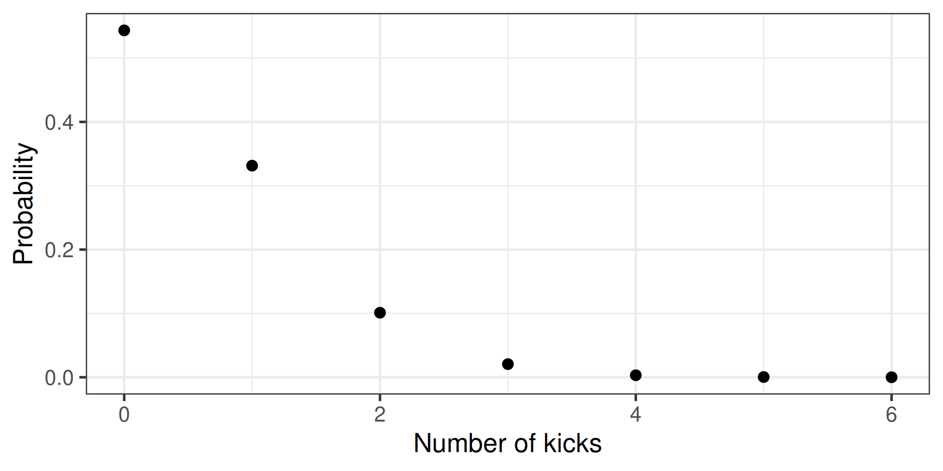
Calculate discrete probability
- E.g., how many people die of horse kicks if there are 0.61 kicks per year
- Described by the Poisson distribution

Two directions
- Calculate the probability
- Randomly sample
Generate a random (Poisson) sample
- E.g., how many people die of horse kicks if there are 0.61 kicks per year
- Described by the Poisson distribution

Two directions
- Calculate the probability
- Randomly sample
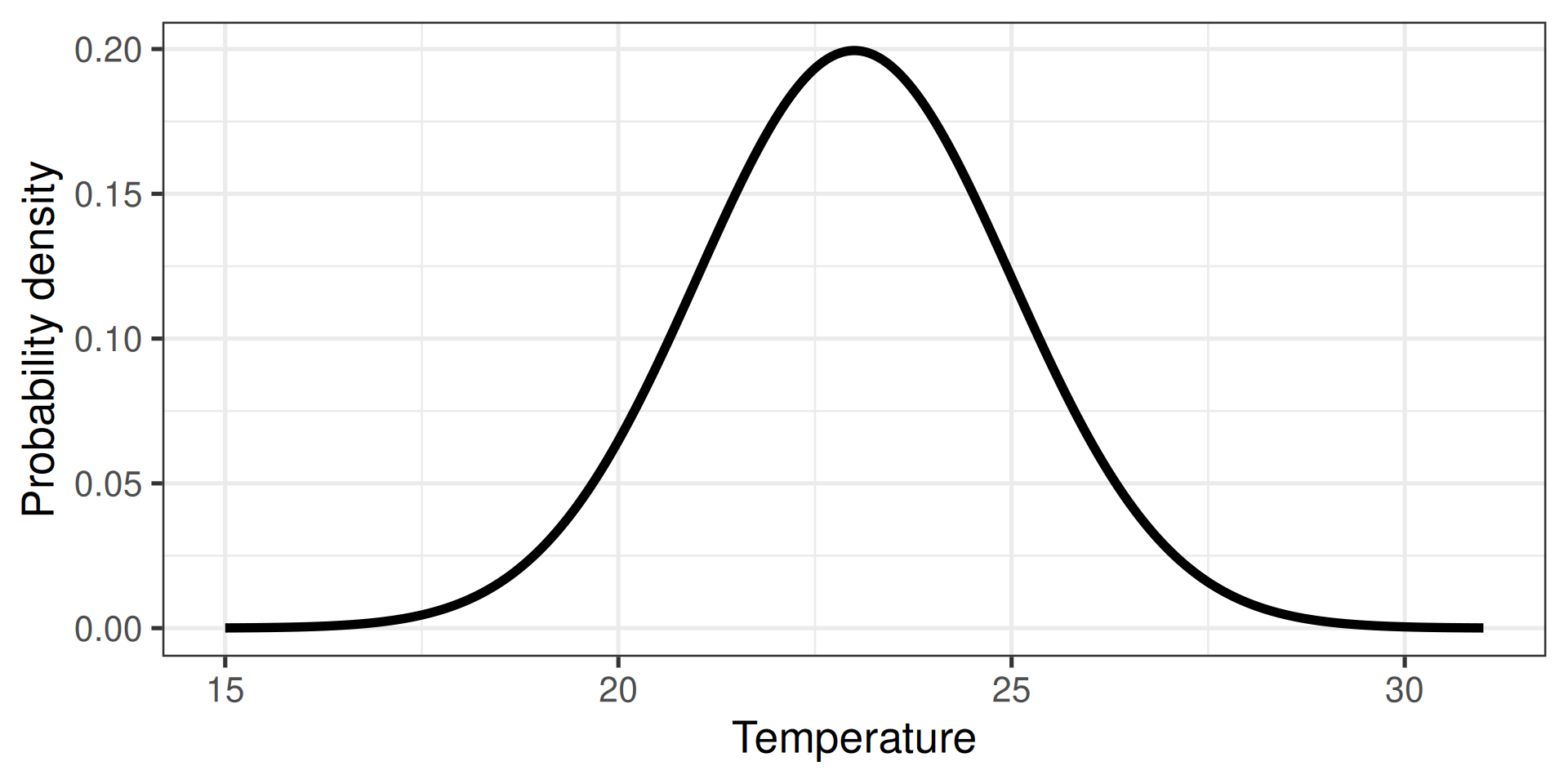
Calculate probability density
- Extension of probabilities to continuous variables
- E.g., the temperature in Stockholm tomorrow
Two directions
- Calculate the probability
- Randomly sample
Generate a random (normal) sample

Two directions
- Calculate the probability
- Randomly sample
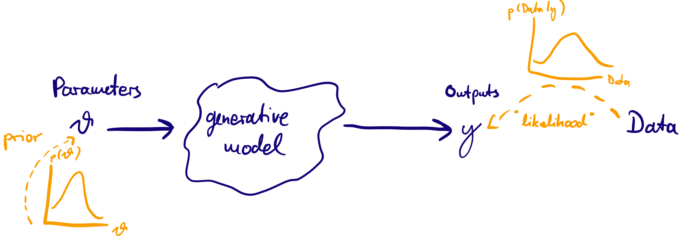
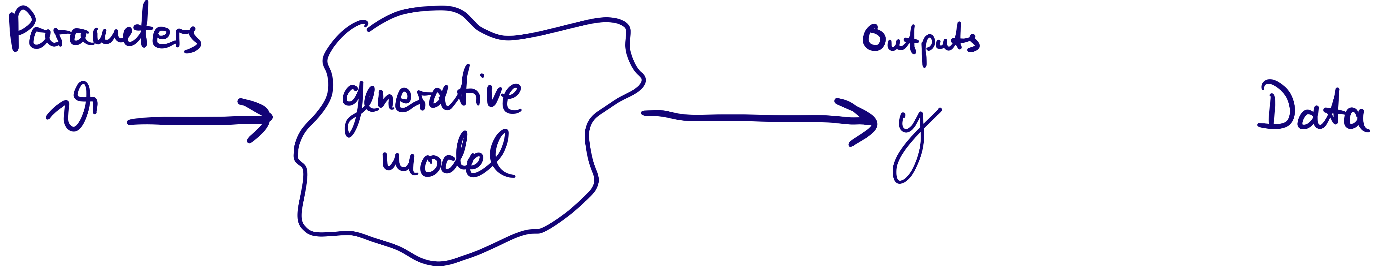
Bayesian inference
The generative model can produce output which looks like data given a set of parameters \(\theta\).
Idea of Bayesian inference: treat \(\theta\) as random variables (with a probability distribution) and condition on data: posterior probability \(p(\theta | \mathrm{data})\) as target of inference.
Bayesian inference