Introduction to statistical concepts used in the course
Why statistical concepts?
We’ll need to estimate things (delays, reproduction numbers, case numbers now and in the future)
We’ll want to correctly specify uncertainty
We’ll want to incorporate our domain expertise
We’ll do this using Bayesian inference
Bayesian inference in 15 minutes

Interlude: probabilities
Probability theory is nothing but common sense reduced to calculation.
Interlude: probabilities (1/3)
- If \(A\) is a random variable, we write \[ p(A = a)\] for the probability that \(A\) takes value \(a\).
- We often write \[ p(A = a) = p(a)\]
- Example: The probability that it rains tomorrow \[ p(\mathrm{tomorrow} = \mathrm{rain}) = p(\mathrm{rain})\]
- Normalisation \[ \sum_{a} p(a) = 1 \]
Interlude: probabilities (2/3)
- If \(A\) and \(B\) are random variables, we write \[ p(A = a, B = b) = p(a, b)\] for the joint probability that \(A\) takes value \(a\) and \(B\) takes value \(b\)
- Example: The probability that it rains today and tomorrow \[ p(\mathrm{tomorrow} = \mathrm{rain}, \mathrm{today} = \mathrm{rain}) = p(\mathrm{rain}, \mathrm{rain})\]
- We can obtain a marginal probability from joint probabilities by summing \[ p(a) = \sum_{b} p(a, b)\]
Interlude: probabilities (3/3)
- The conditional probability of getting outcome \(a\) from random variable \(A\), given that the outcome of random variable \(B\) was \(b\), is written as \[ p(A = a | B = b) = p(a| b) \]
- Example: the probability that it rains tomorrow given that it rains today \[ p(\mathrm{tomorrow} = \mathrm{rain} | \mathrm{today} = \mathrm{rain}) = p(\mathrm{rain} | \mathrm{rain})\]
- Conditional probabilities are related to joint probabilities as \[ p(a | b) = \frac{p(a, b)}{p(b)}\]
- We can combine conditional probabilities in the chain rule \[ p(a, b, c) = p(a | b, c) p(b | c) p (c) \]
Probability distributions (discrete)
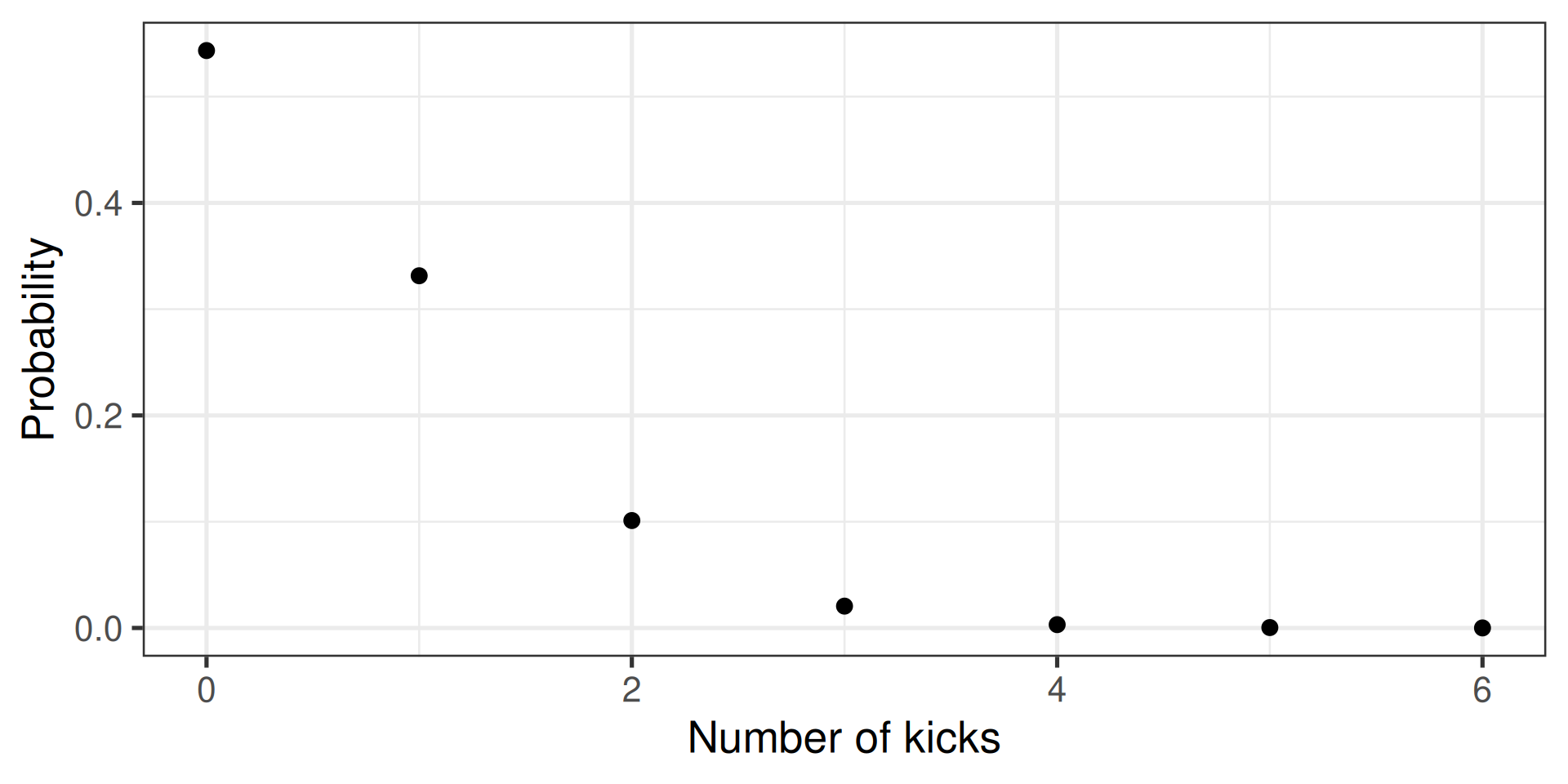
- E.g., how many people die of horse kicks if there are 0.61 kicks per year
- Described by the Poisson distribution
Two directions
- Calculate the probability
- Randomly sample
Calculate discrete probability
- E.g., how many people die of horse kicks if there are 0.61 kicks per year
- Described by the Poisson distribution
Two directions
- Calculate the probability
- Randomly sample
Generate a random (Poisson) sample
- E.g., how many people die of horse kicks if there are 0.61 kicks per year
- Described by the Poisson distribution
Two directions
- Calculate the probability
- Randomly sample
Probability distributions (continuous)
- Extension of probabilities to continuous variables
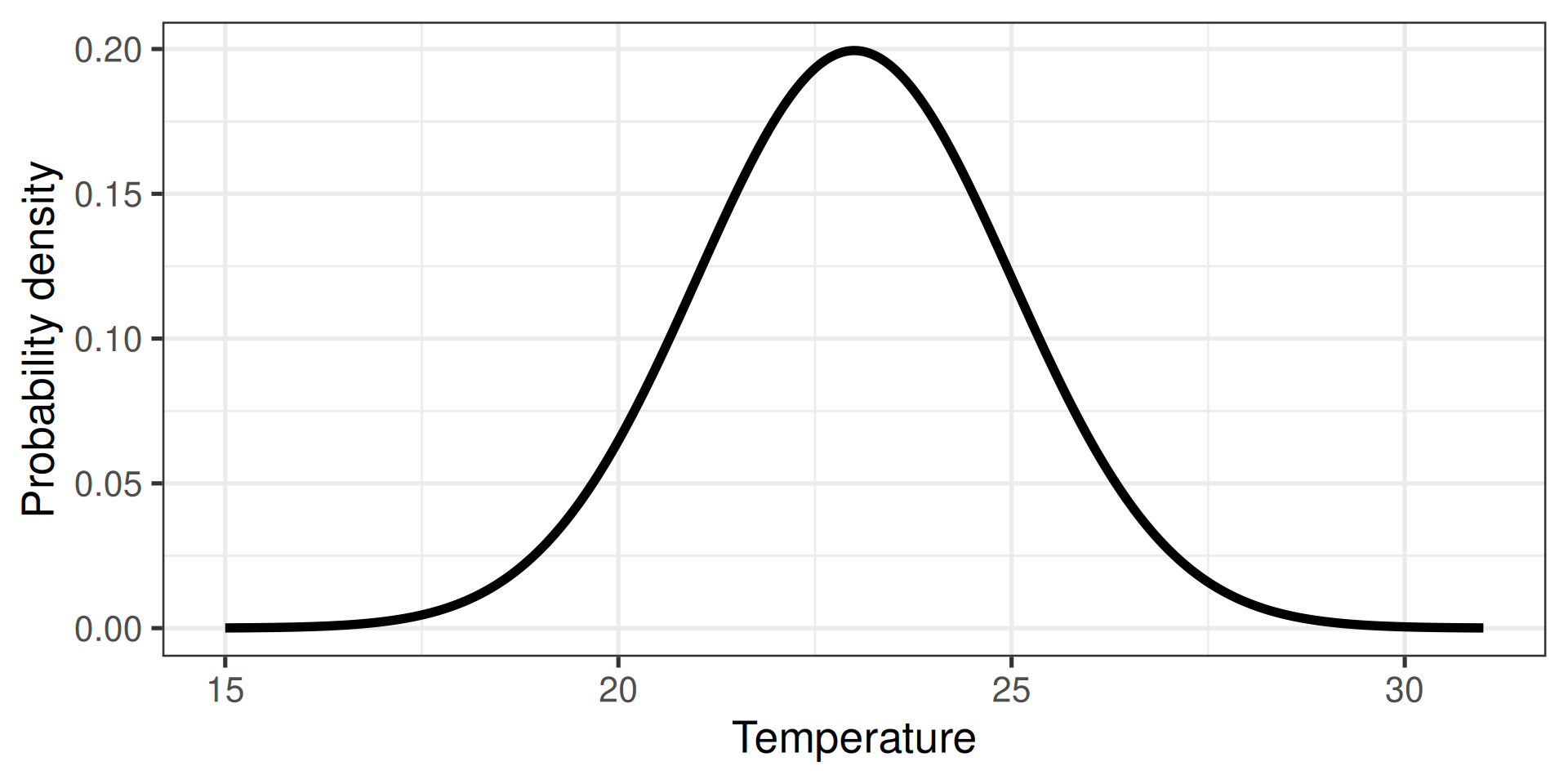
- E.g., the temperature in Stockholm tomorrow
Normalisation: \[ \int p(a) da = 1 \]
Marginal probabilities: \[ p(a) = \int_{} p(a, b) db\]
Two directions
- Calculate the probability (density)
- Randomly sample
Calculate probability density
- Extension of probabilities to continuous variables
- E.g., the temperature in Stockholm tomorrow

Two directions
- Calculate the probability
- Randomly sample
Generate a random (normal) sample

Two directions
- Calculate the probability
- Randomly sample
Bayesian inference in 15 minutes

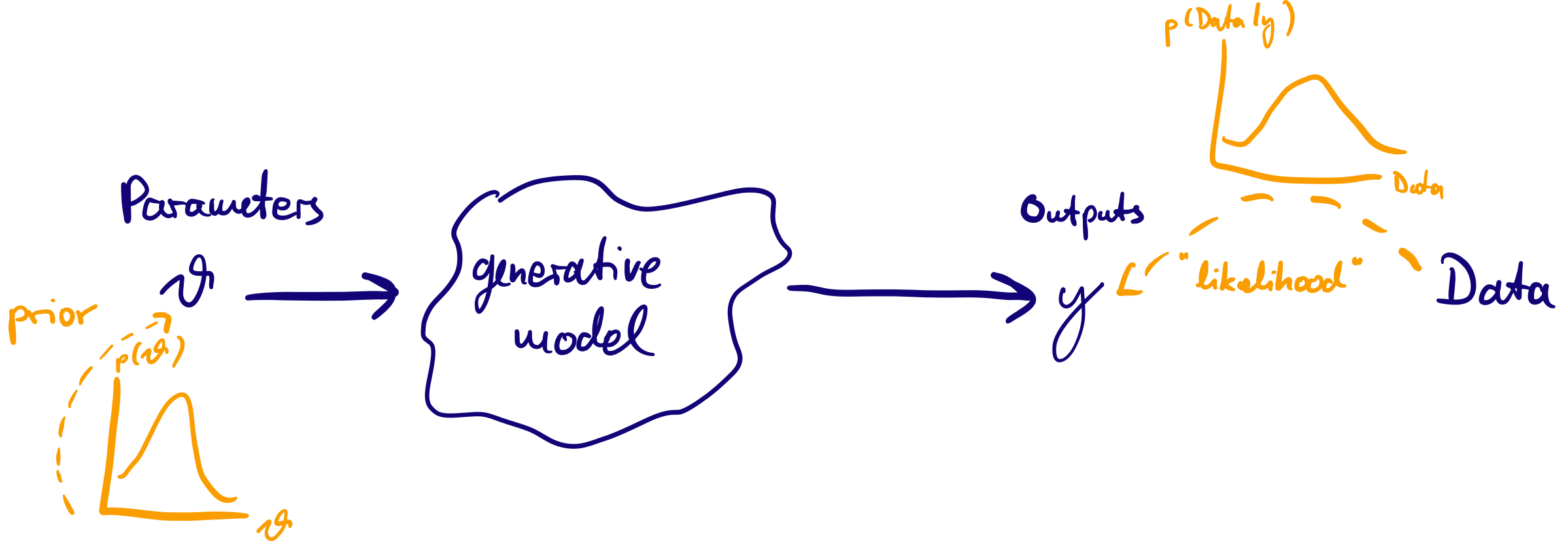
Idea of Bayesian inference: treat \(\theta\) as random variables (with a probability distribution) and condition on data: posterior probability \(p(\theta | \mathrm{data})\) as target of inference.
Bayes’ rule
- We treat the parameters of the a \(\theta\) as random with prior probabilities given by a distribution \(p(\theta)\). Confronting the model with data we obtain posterior probabilities \(p(\theta | \mathrm{data})\), our target of inference. Applying the rule of conditional probabilities, we can write this as
\[ p(\theta | \textrm{data}) = \frac{p(\textrm{data} | \theta) p(\theta)}{p(\textrm{data})}\]
\(p(\textrm{data} | \theta)\) is the /likelihood/
\(p(\textrm{data})\) is a /normalisation constant/
In words, \[\textrm{(posterior)} \propto \textrm{(normalised likelihood)} \times \textrm{(prior)}\]
Bayesian inference

MCMC
Markov-chain Monte Carlo (MCMC) is a method to generate samples from the posterior distribution, the target of inference
stan is a probabilistic programming language that helps you to write down probabilistic models and to fit them using MCMC samplers and other methods.
Introduction to statistical concepts used in the course

