Baselines and seasonality
Persistence & mean
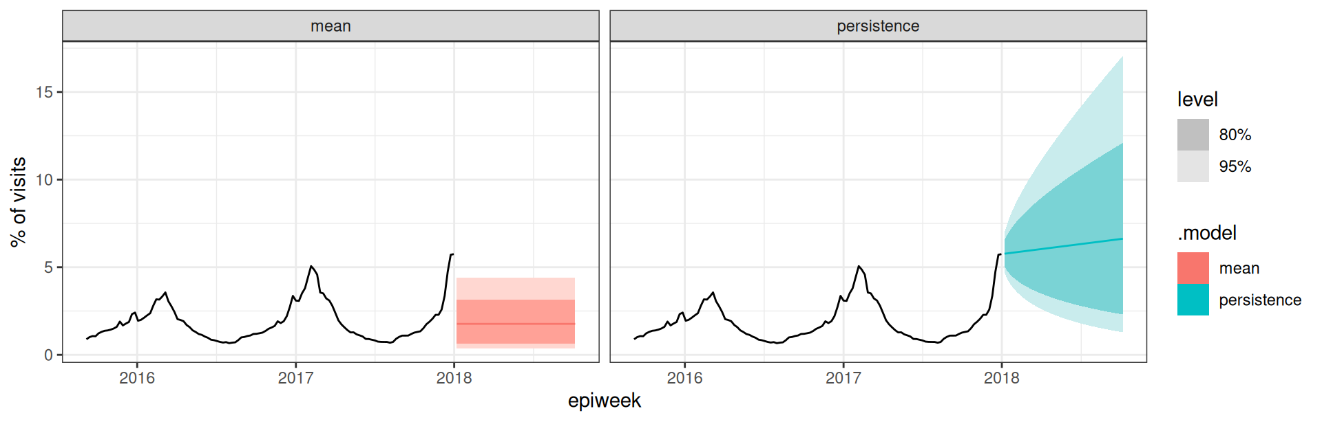
Persistence extends the last value; the mean ignores where we are.
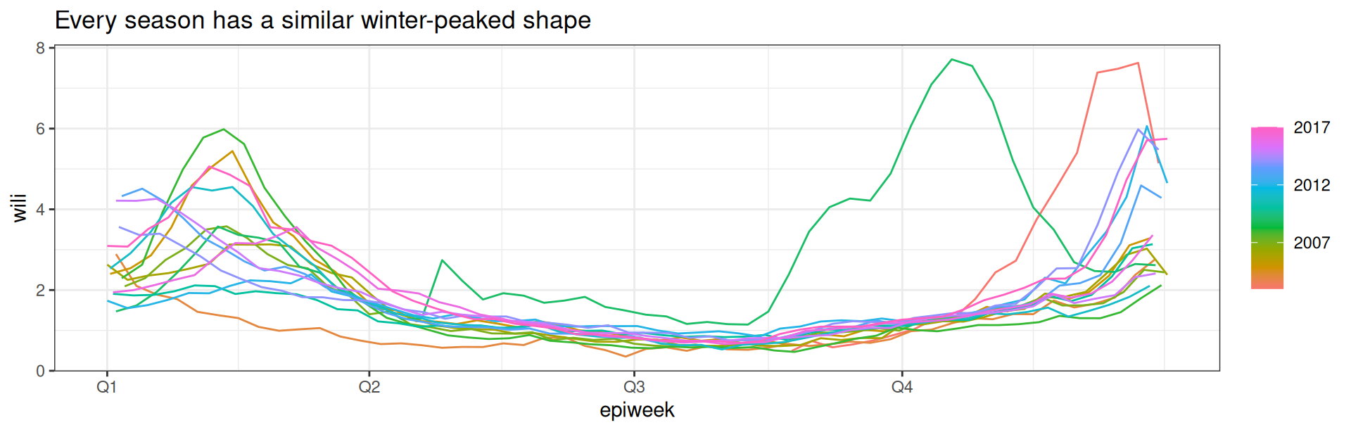
The data are seasonal
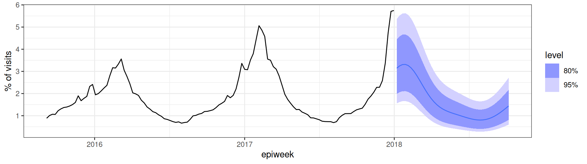
A seasonal baseline: harmonic regression
ARIMA(y ~ pdq(0,0,0) + fourier(period = "year", K = 3))
- No AR / differencing / MA — only sine & cosine curves with a 1-year period
- Forecast = a smooth “seasonal climatology”; still ignores the most recent weeks
Improving on the baselines
ARIMA(y ~ pdq(2,0,0) + fourier(period = "year", K = 3))
- AR(2) anchors to recent values; Fourier pulls toward the seasonal shape
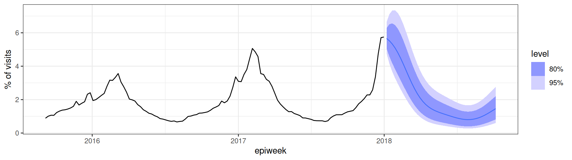
All together
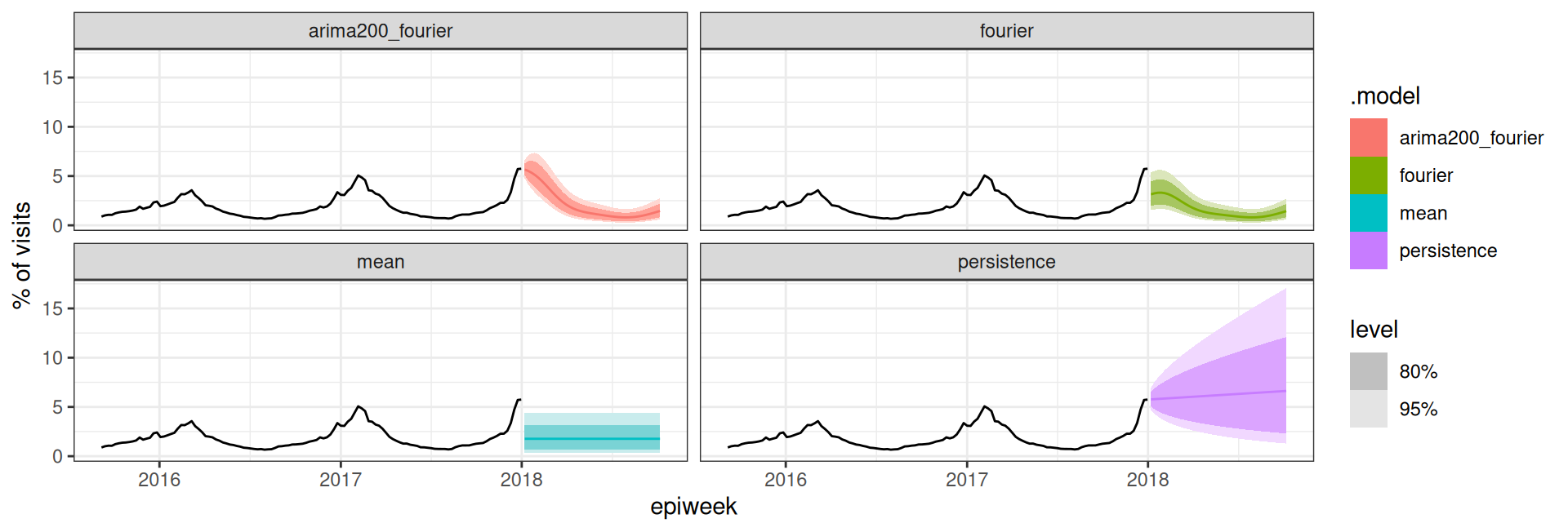
The combined model captures the seasonal shape and starts from the right level — but “looks better” isn’t proof.
Did it work? Check the residuals
If a model captured the structure, its residuals should look like white noise — flat ACF, especially at the seasonal lag ~52.
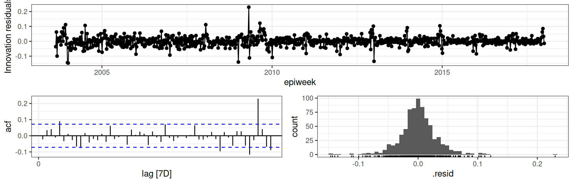
What we want to see
- top panel: white noise in the residuals
- bottom left: no significant residual autocorrelation
- bottom right: Normal, symmetric distrbution of residuals