Epidemiologically-motivated forecasting

Forecasting & evaluation of infectious disease dynamics

Forecasting so far

In earlier sessions we used statistical models such as ARIMA that find patterns in the reported series and project them forward.

What we model

  • The reported series (case counts or percentages)
  • Trends and seasonality
  • Autocorrelation in the data

What we ignore

  • How infections arise
  • Generation time / transmission
  • Susceptible depletion

From infections to infections: the generation time

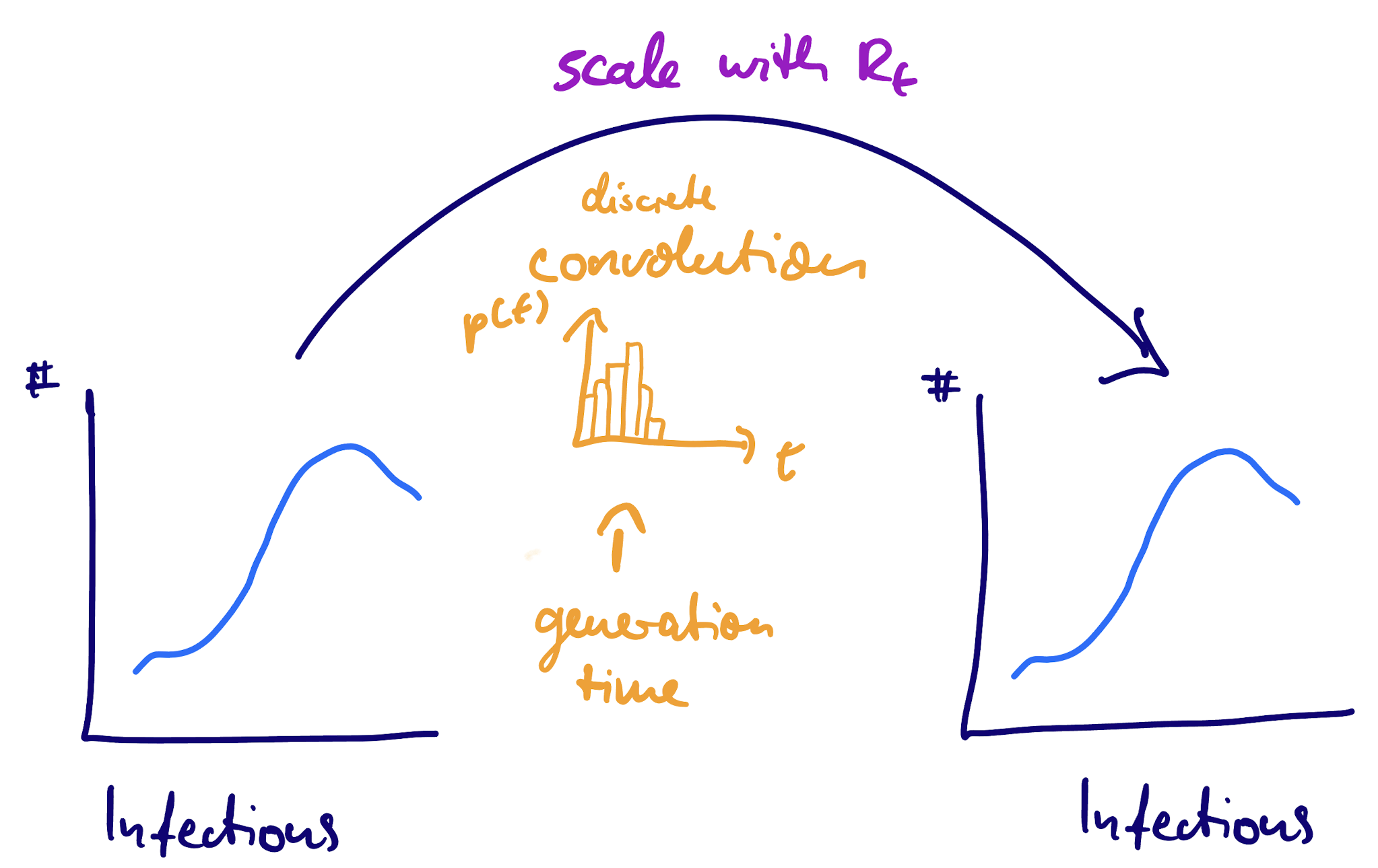
The time from one infection (person A) to the next infection it causes (person B) is the generation time, a distribution \(g(t)\).

It describes how the infections caused by one person are spread out over the days after they are infected.

The renewal equation as a convolution

Infections today depend on infections in the past, weighted by the generation-time distribution and scaled by \(R_t\).

\[ I_t = R_t \times \sum_{t' < t} I_{t'}\, g(t - t') \]

A renewal equation is an epidemiologically-informed autoregression

ARIMA

\[ y_t = \sum_s \phi_s\, y_{t-s} + \varepsilon_t \]

  • Coefficients \(\phi_s\) are free parameters
  • \(\varepsilon_t\) is an additive noise term

Renewal

\[ I_t = \sum_s R_t\, w_s\, I_{t-s} + \iota_t \]

  • Coefficient is \(R_t\, w_s\), reproduction number times generation-time weight
  • \(\iota_t\) (imports) sits where the ARIMA has \(\varepsilon_t\), set to zero here
  • Fitting adds a negative binomial observation model on top

From infection to report: delays

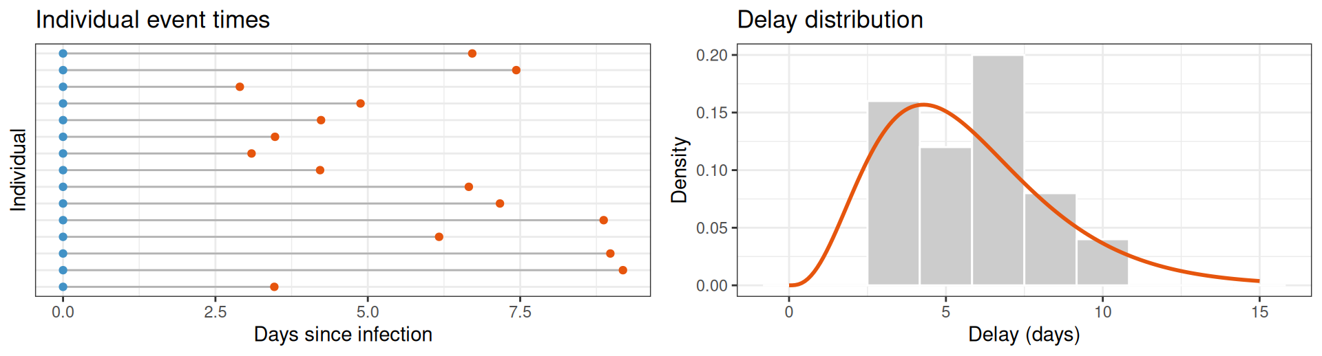
We never observe infections directly. Each infected person is reported some days later, after an incubation period and a reporting delay. Individual delays vary, and together they form a delay distribution.

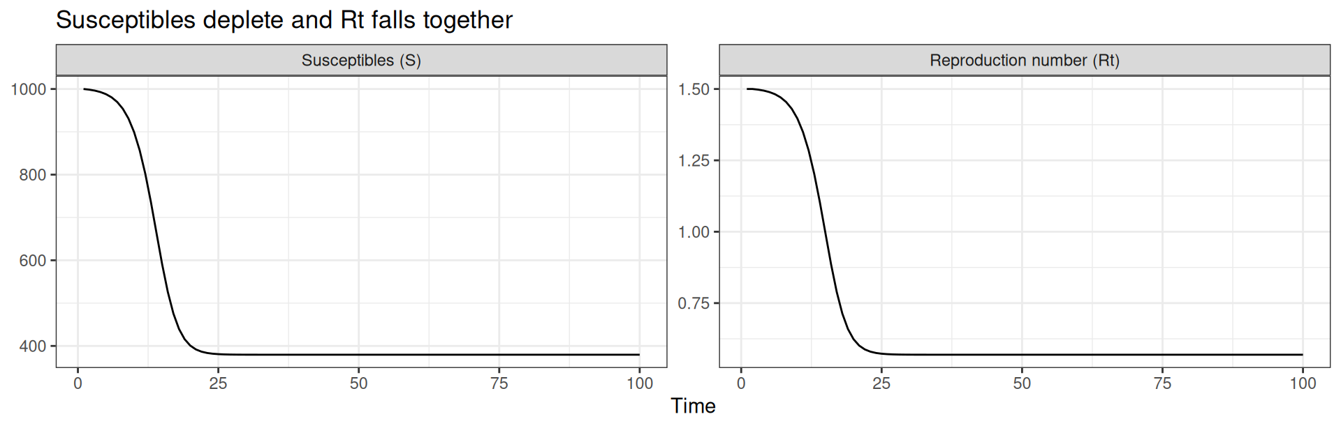
Adding mechanism: susceptible depletion

The population at risk is finite.

As susceptibles run out, the effective reproduction number falls below \(R_0\) even with no change in behaviour.

\[ R_t = \frac{S_{t-1}}{N}\, R_0 \]

EpiNow2

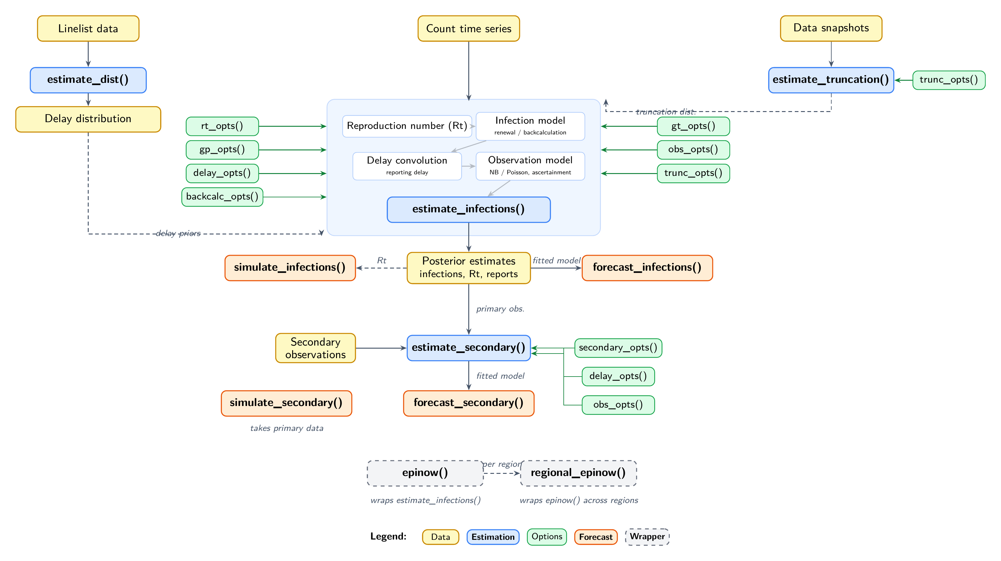
estimate_infections() fits the renewal infection model, the delay convolution, and the observation model together in Stan.

Your turn

  1. Fit a renewal model and the ARIMA baseline for a single forecast before the peak.
  2. Compare five models, turning the \(R_t\) and population knobs, across 12 forecast dates.
  3. Score them on the natural and log scale, and see where mechanism matters most.
  4. Misinform a model with the wrong population and see the cost.
Return to the session