Time Series Forecasting 101

Forecasting & evaluation of infectious disease dynamics

Which Model to Use?

There are many types of models available to us:

  • A range of choices from mechanistic to purely statistical.

  • Bayesian, frequentist, machine learning.

  • Stochastic vs. Deterministic

How should we decide which model(s) to incorporate for nowcasting and forecasting?

What outputs and features do we require of these models?

Using Data to Inform Modeling Choices

Often, what motivates one’s modeling choices are the trends and patterns observed in the data.
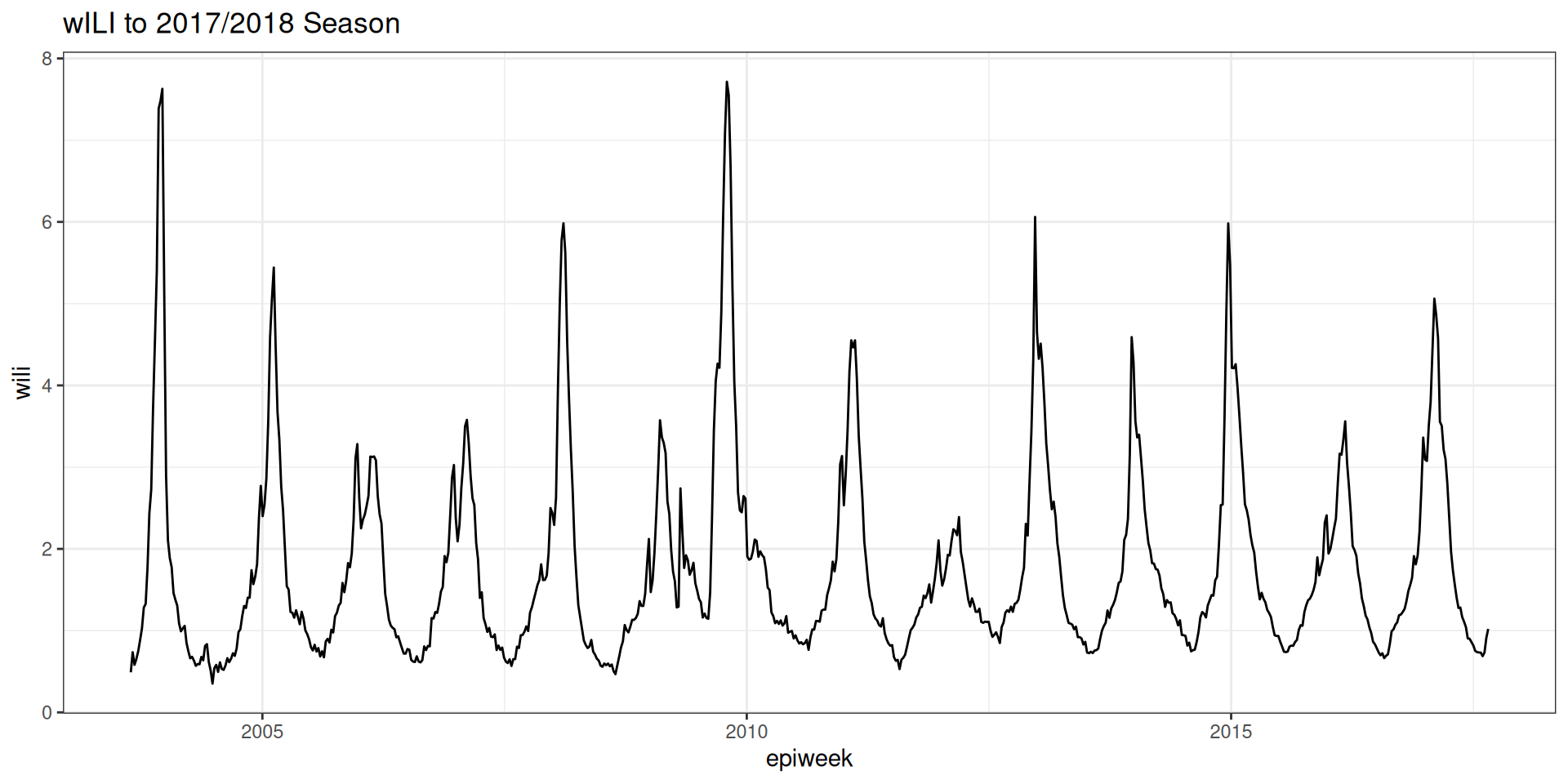
Features we cover in this session

  • Auto correlation
  • Partial auto-correlation
  • Stationarity
  • Constant variance

Autocorrelation

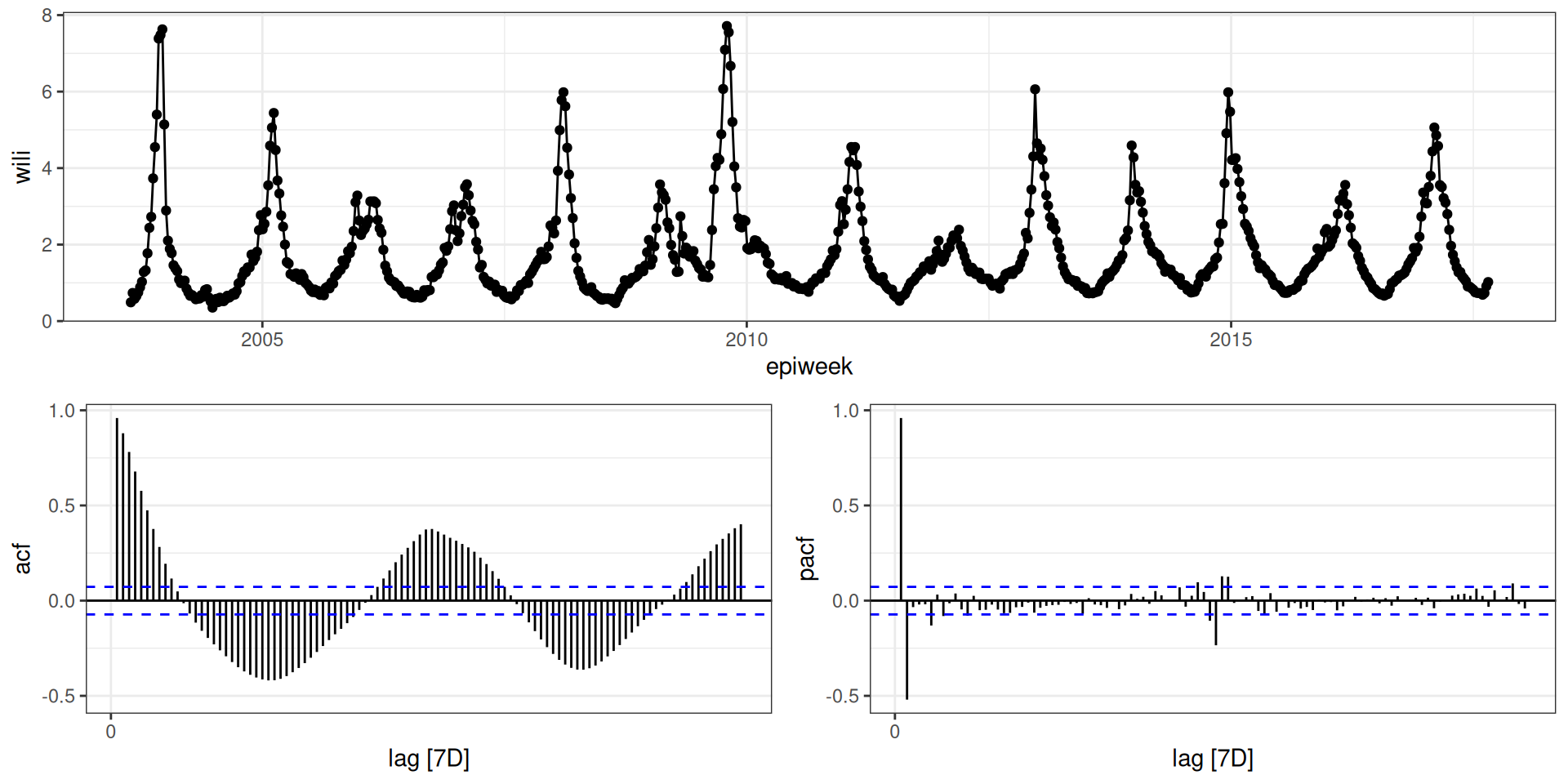
Autocorrelation and Partial Autocorrelation (ACF/PACF) plots measure the linear relationship between lagged values of a time series.
Describing autocorrelation

ACF plots correlation of \(y_t\) and \(y_{t-k}\) as a function of k.

Correlations show periodicity of ~52 weeks.
Describing partial correlation

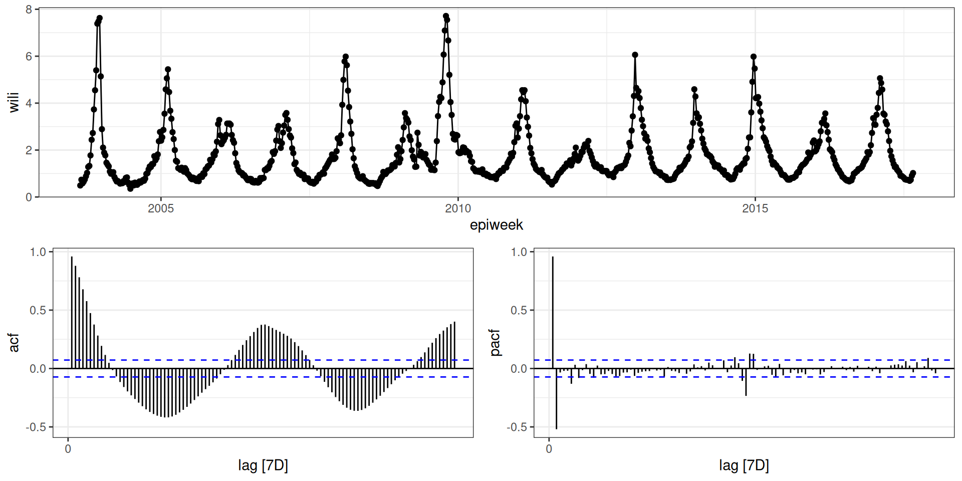
PACF plots correlation of \(y_t\) and \(y_{t-k}\) as a function of k, adjusted for shorter lags.

Only a few partial correlations are significant.
Stationarity

Definition

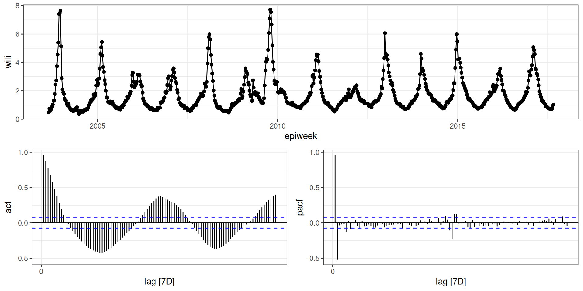
A time series is stationary if the mean and variance of the data do not change over time.

Implications in practice

Stationarity means that there are no long-term predictable patterns in a time-series, but there can still be predictability in the short term.

Assumption

ARIMA (and other models) assume data are stationary (won’t work as well if data are not).

Seasonality

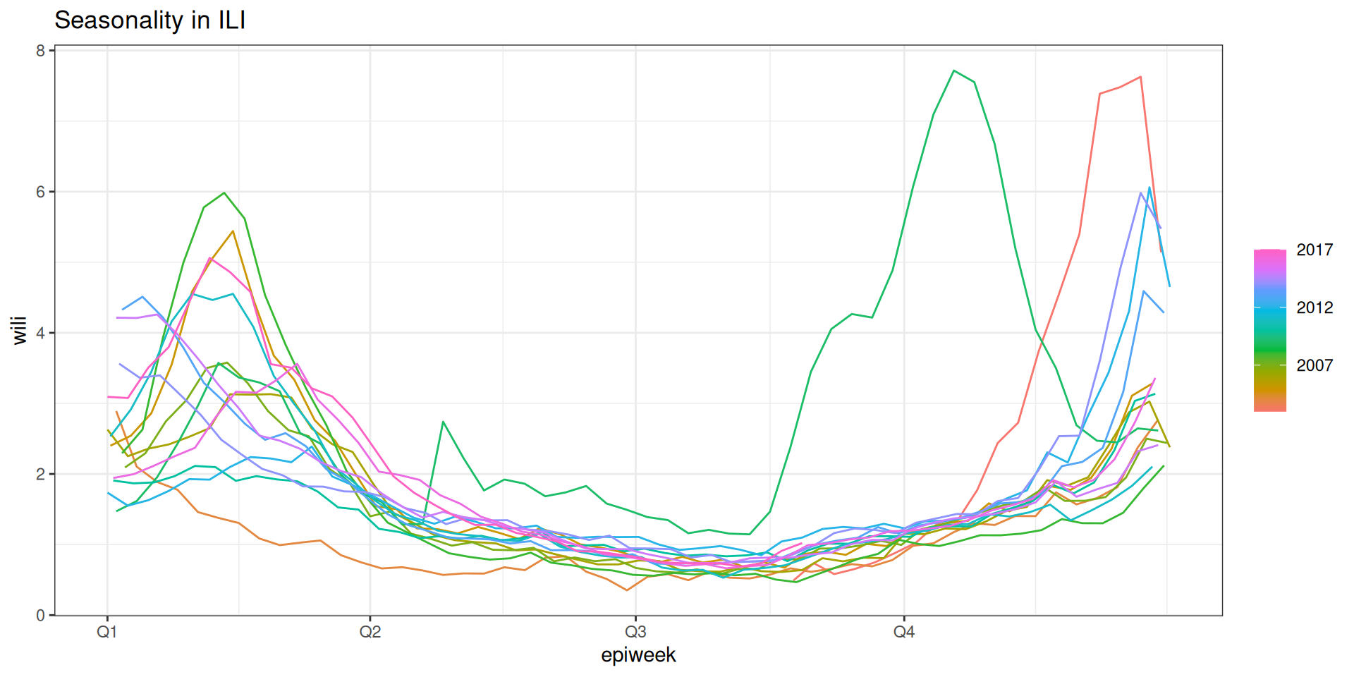
Seasonal patterns are common with many (but not all) endemic diseases. Seasonality can make a disease more predictable, but also means it’s not stationary.
Constant variance

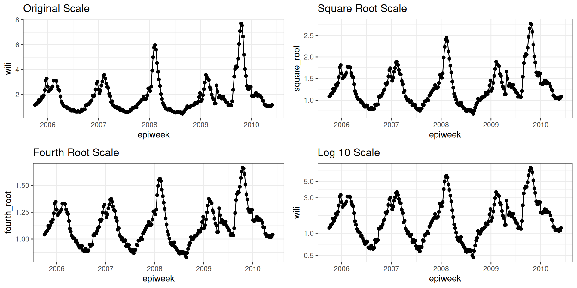
A key assumption of many models is constant variance over time. Transformations often help.
Time-series Regression Models: ARIMA

Widely used for decades!

Notation is \(ARIMA(p, d, q).\)

  • AR (Auto-Regressive order \(p\))
    • Uses past values to predict current ones.
    • Useful when there is auto-correlation.
  • I (Integrated order \(d\))
    • Differences (\(y_t - y_{t-1}\)) help make the series stationary.
    • Useful when there is non-stationarity.
  • MA (Moving Average order \(q\))
    • Uses recent model residuals as predictors.

Figuring out which \((p,d,q)\) to use is tricky!

A Lag-1 model: ARIMA(p=1,d=0,q=0)

Here is the equation for an ARIMA(1,0,0) model: \[ y_t = \mu_t + \phi_1 y_{t-1} + \varepsilon_t \]

  • \(\mu_t\) is a constant (like an intercept term in the regression)
  • \(\phi_1\) is a coefficient for the auto-regressive term
  • \(\varepsilon_t\) is a random error term with mean zero and constant variance

Warning

Note the constant variance assumption!

A Random Walk model: ARIMA(p=0,d=1,q=0)

Here is the equation for an ARIMA(0,1,0) model: \[y_t - y_{t-1} = \varepsilon_t \qquad\Longleftrightarrow\qquad y_t = y_{t-1} + \varepsilon_t\]

Tip

No AR terms (\(p=0\)), one difference (\(d=1\)), no MA terms (\(q=0\)). The model sees the first differences as white noise.

ARIMA(p=1,d=1,q=0)

Here is an equation for an ARIMA(1,1,0) model: \[ y_t - y_{t-1} = \phi_1 (y_{t-1} - y_{t-2}) + \varepsilon_t.\]

Note

This model is the same as the last slide but here both the “outcome” variable and predictor variable is now a first-order difference of \(y_t\), corresponding to the second “1” in (1,1,0).

Your Turn

  1. Explore the influenza dataset, focusing on assessing observed patterns qualitatively and quantitatively.
  2. Explore different ways of improving modeling forecasts by incorporating patterns observed in data into our models.

Return to the session