Nowcasting and forecasting of infectious disease dynamics
Building models iteratively
In this course we have been building models iteratively — each session added a piece and checked it.
This is the Bayesian workflow
A Bayesian workflow is the iterative loop of building, checking, and revising a model.
Bayesian Workflow (Gelman et al., 2026)
The workflow loop
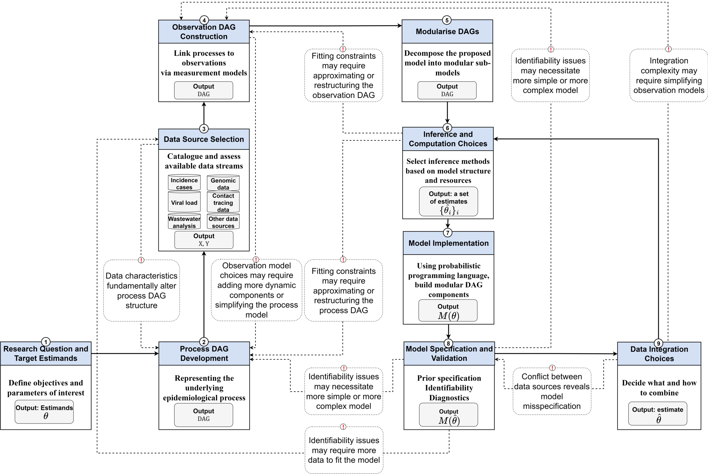
A workflow for infectious disease modelling
A workflow for infectious disease modelling. Figure by Abbott et al. (MIT licence).
Reading the workflow
Question & estimands — infections and \(R_t\)
Process model
Process model — one shared renewal process
Data source selection
Data source selection — catalogue each data source and how it is biased
Observation model per source
Observation model per source — a delay + a scaling + a likelihood
What is a DAG?
A directed acyclic graph draws a model as a picture. Each quantity is a node, and an arrow runs from a quantity to whatever it generates.
Read top to bottom, it traces how the data come about
The arrows make the model’s conditional independence assumptions explicit
The DAG is the TLDR of the model.
Modularise
Modularise — split into sub-models that can be checked on their own
Inference & computation choices
Inference & computation choices — how to fit the model
Implementation
Implementation — write the model
Model validation
Model validation — check each piece against data
Data integration
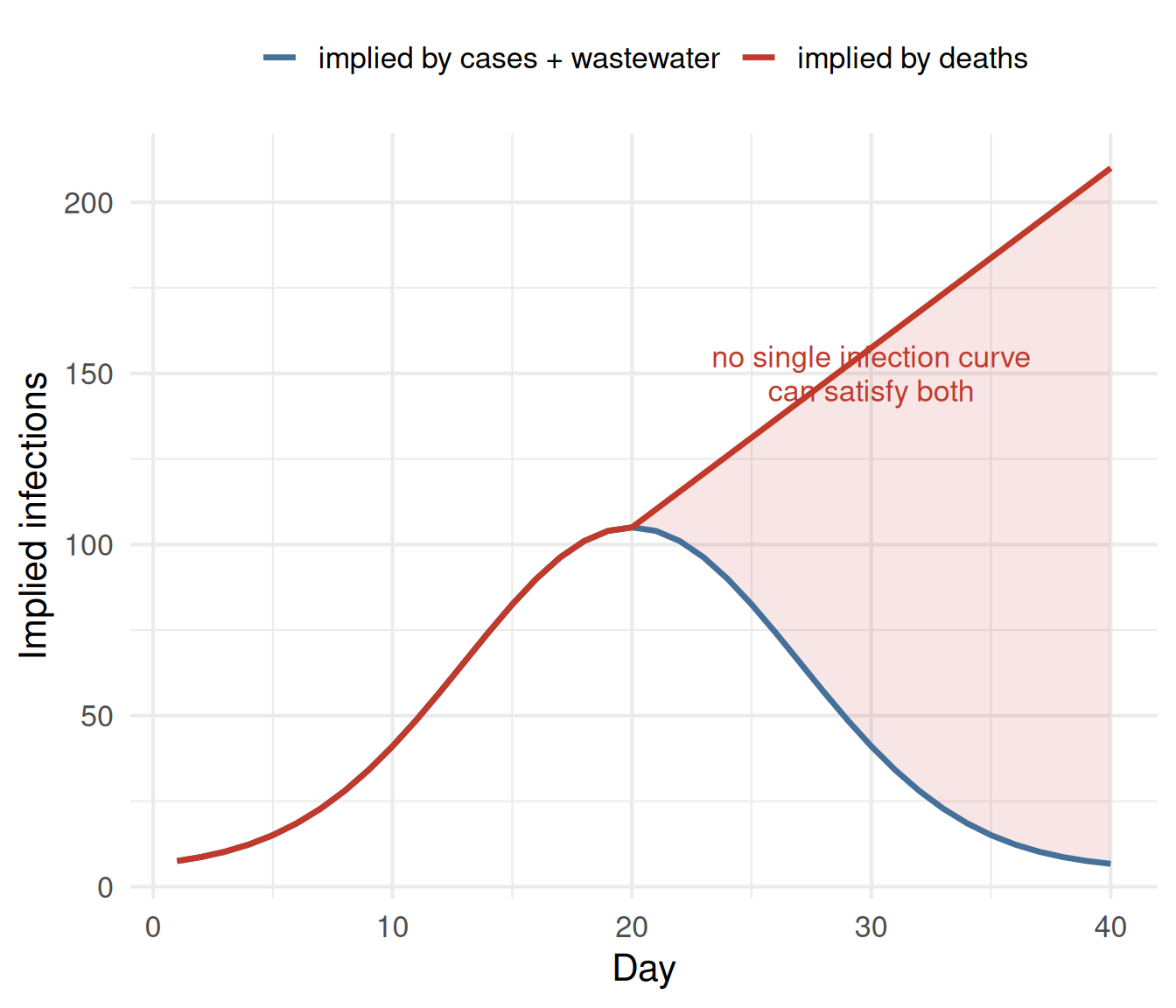
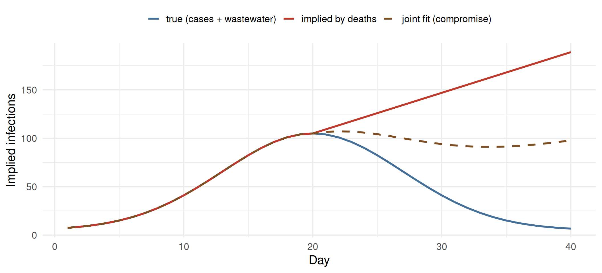
Data integration — how to combine the data sources; conflict reveals misspecification
The question
Our target is unchanged: recover the latent infections and \(R_t\) as quickly and with as little bias as we can.
Now we introduce our data sources
To answer that question we bring in several data sources at once, each a delayed, scaled view of the same infections:
Cases — timely, but depend on testing; only a fraction ascertained
Deaths — stable, but long-delayed and severity-dependent
Wastewater — independent of care-seeking; thought to lead cases, but indirect, noisy, and on its own scale
Wastewater: a tangent
What is wastewater surveillance?
Measuring pathogen RNA shed into sewage — a population-level signal.
Why people are interested:
Does not depend on testing, care-seeking, or ascertainment
Thought to lead case reports, and picks up asymptomatic infection
Relatively cheap at scale (one sample covers a whole catchment)
Challenges: it is noisy and indirect, and needs scaling / normalisation before it can be compared to infections.
A DAG for wastewater
From infections to what we measure:
Back to joint modelling
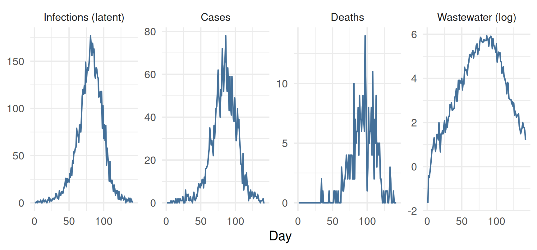
Three data sources from one trajectory
Each data source is a delayed, rescaled echo of the same infection curve.
Steps 2–4 in one picture
We defined the question (step 1). This is steps 2–4: the shared process, the data sources, and an observation model for each — every data source a convolution of the shared latent infections, conditionally independent given \(I\).