Jointly fitting multiple data streams
One outbreak, several views
So far: estimate \(R_t\) from a single observed time series.
In reality we watch an outbreak through several streams at once:
- Cases — timely, but depend on testing; only a fraction ascertained
- Deaths — stable, but long-delayed and severity-dependent
- Wastewater — does not depend on care-seeking, but indirect and on its own scale
Each is a delayed, scaled view of the same infections.
The question
Our target is unchanged: recover the latent infections and \(R_t\), as timely and as well-anchored as we can.
- Cases track the timing of recent infections, but carry reporting noise and tell us only an ascertained fraction.
- Deaths are sparser and badly lagged, so they say little about the present, but anchor the longer-term level.
- Wastewater is independent of care-seeking, but indirect and on its own scale.
Alone, none pins down both the infection level and \(R_t\).
What does each stream add, and what happens when they pull in different directions?
What is wastewater surveillance?
Measuring pathogen RNA shed into sewage — a population-level signal.
Why people are interested:
- Does not depend on testing, care-seeking, or ascertainment
- Can lead case reports, and picks up asymptomatic infection
- Relatively cheap at scale (one sample covers a whole catchment)
Challenges: it is noisy and indirect, and needs scaling / normalisation before it can be compared to infections.
This is why it is attractive as a third, parallel stream.
Don’t reach for the whole model at once
Fitting several streams is one step in a wider modelling workflow.
A Bayesian workflow is the iterative loop of building, checking, and revising a model — never a single leap to the final model.
[Placeholder: cover of Aki Vehtari et al.’s Bayesian workflow book — to be added]
We let that general idea drive how we develop this model.
A workflow for infectious disease modelling
The infectious-disease-specific instance of that loop:
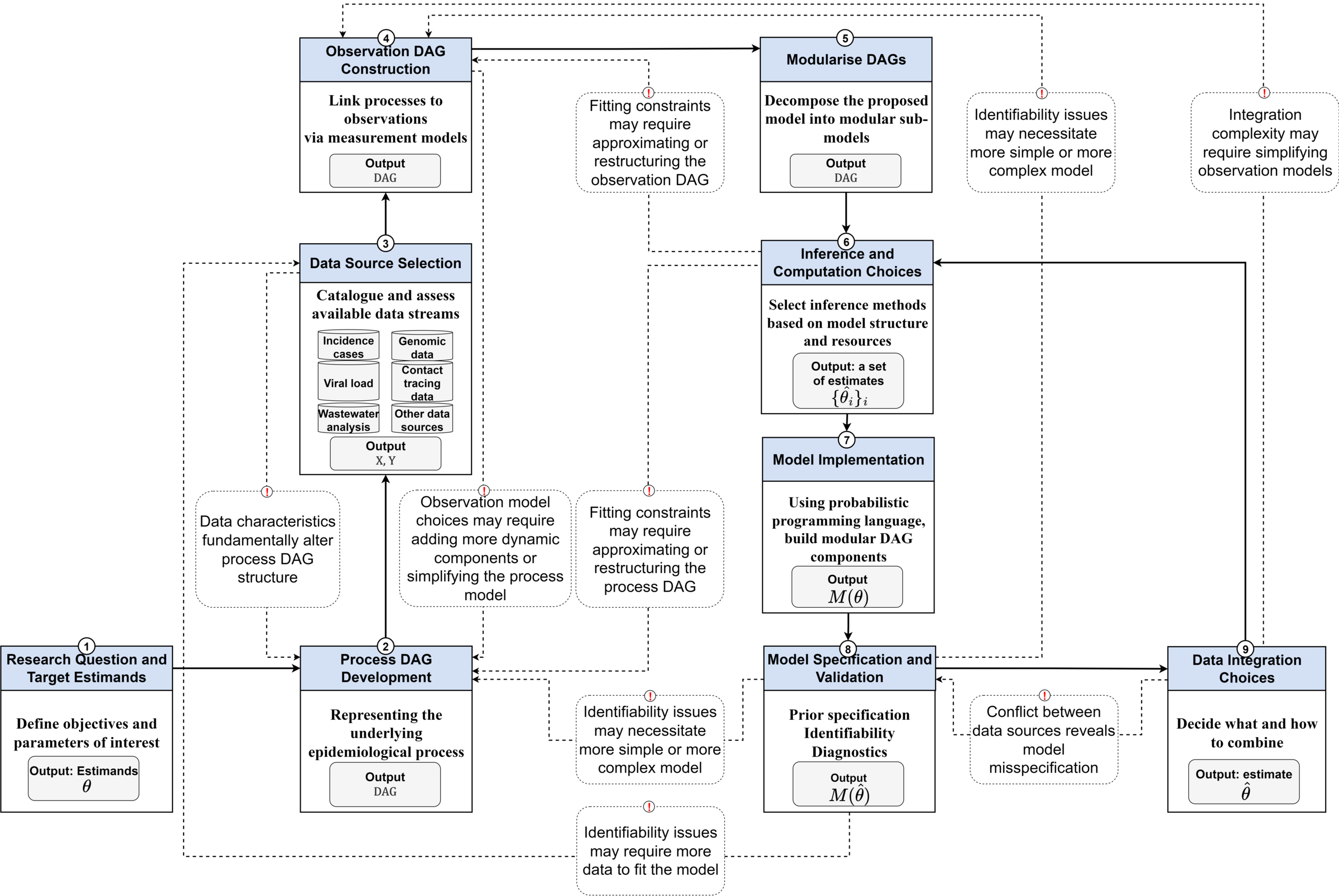
Reading the workflow, bottom-left up
- Question & estimands — infections and \(R_t\)
- Process model — one shared renewal process
- Data source selection — what each stream measures, and its biases
- Observation model per source — a delay + a scaling + a likelihood
- Data integration — how to combine them (the key choice)
- Inference, checking & iteration — fit, check (PPCs, conflict), revise
A shared process, a swappable observation model per stream — so we can build it in parts.
Three streams from one trajectory
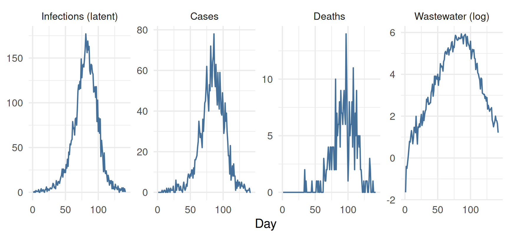
Each stream is a delayed, rescaled echo of the same infection curve.
Parallel observation of shared infections
One way to combine them: every stream is its own convolution of the shared latent infections, conditionally independent given \(I\).
\[ \text{cases}_t \sim f\big(\text{convolve}(I, p_\text{cases})\big), \quad \text{deaths}_t \sim g\big(\text{convolve}(I, p_\text{deaths})\big) \]
Infections become the one shared quantity that every stream informs.
Build it in parts
One Stan model, three use_* switches — fit any subset of streams:
- Each stream on its own — does it recover infections through its delay and scaling?
- Link two streams — cases + deaths share one infection process
- Add the third — wastewater too; infections and \(R_t\) informed by all
- Stress-test — what happens when streams conflict?
What each stream buys you
- Cases pin down the recent trajectory (short delay)
- Deaths are uncertain near the present (long delay), but anchor the level
- Together they constrain infections better than either alone
But the absolute level stays weakly identified: streams constrain infections \(\times\) scaling, not each separately. (The workflow’s identifiability arrow.)
When streams conflict
Each stream implies its own answer to “what did infections look like?”.
Streams conflict when those implied trajectories can’t both come from one \(R_t\) path:
- changing ascertainment (testing policy)
- mis-specified delays or scalings (e.g. drifting IFR)
- genuinely different populations
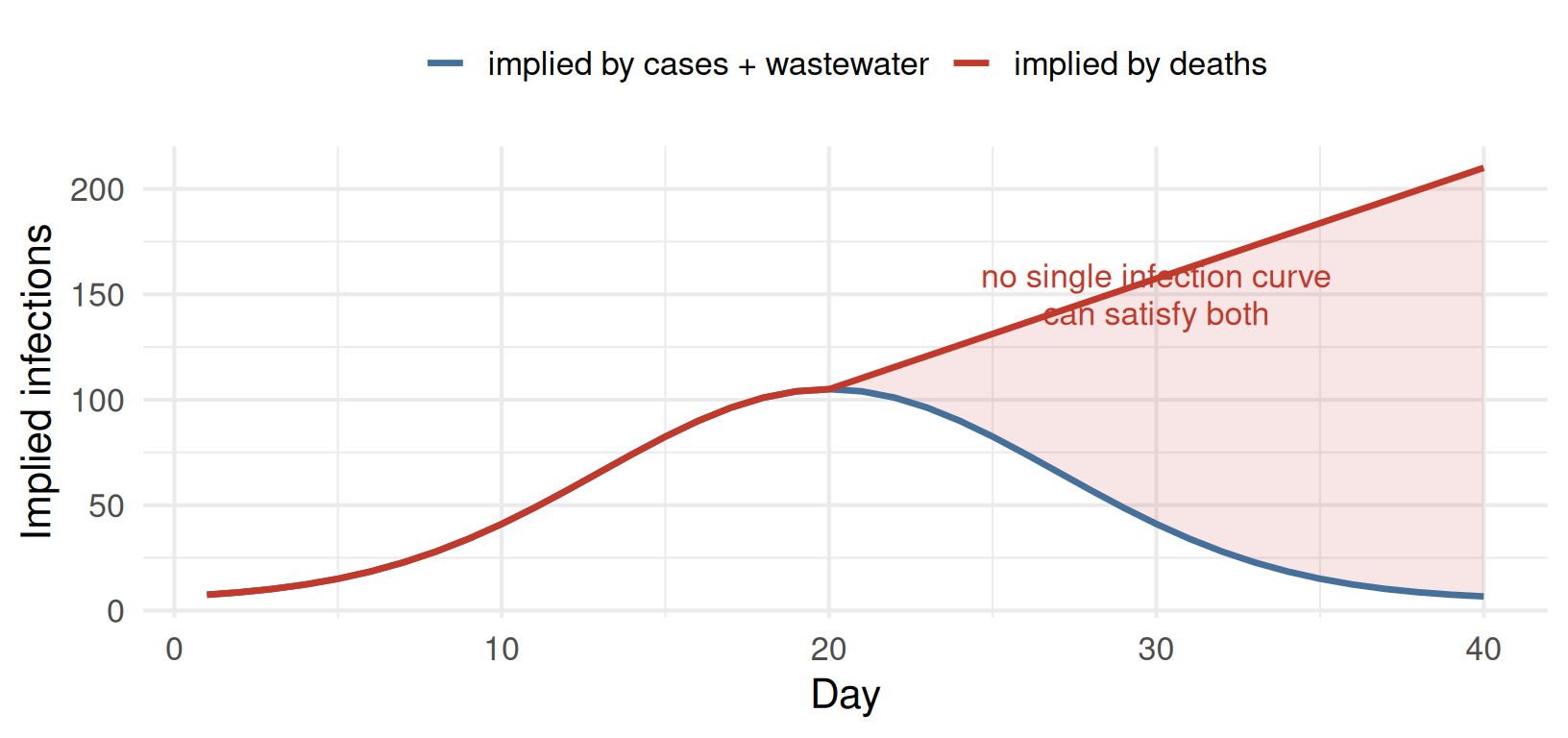
Conflict distorts the joint fit
A single shared \(I\) can’t be both falling (cases, wastewater) and rising (deaths), so the model splits the difference — and \(R_t\) is faithful to no stream.
It surfaces in three linked ways:
- Poor fit to one stream (posterior predictive check)
- Tension in the shared infections (distorted, more uncertain)
- Degraded sampling (divergences, low ESS, high
rhat)
Resolving conflict
A shared latent process surfaces conflict and gives a compromise — it does not resolve it.
Genuine resolution = model the reason the streams disagree:
- Diagnose, don’t average — which stream, which assumption?
- Relax the offending assumption — e.g. time-varying ascertainment / IFR
- Compare models — does the conflict resolve?
- Down-weight or drop — last resort, only once you know why
This loop is the modelling workflow.
Your Turn
- Simulate parallel streams from one shared infection trajectory
- Fit each stream alone, then link them through the shared infections
- Recover infections and \(R_t\) from the joint fit
- Make the deaths conflict, see the joint model surface it, then resolve it by modelling the mechanism
Jointly fitting multiple data streams