Delay distributions at the population level
Nowcasting and forecasting of infectious disease dynamics
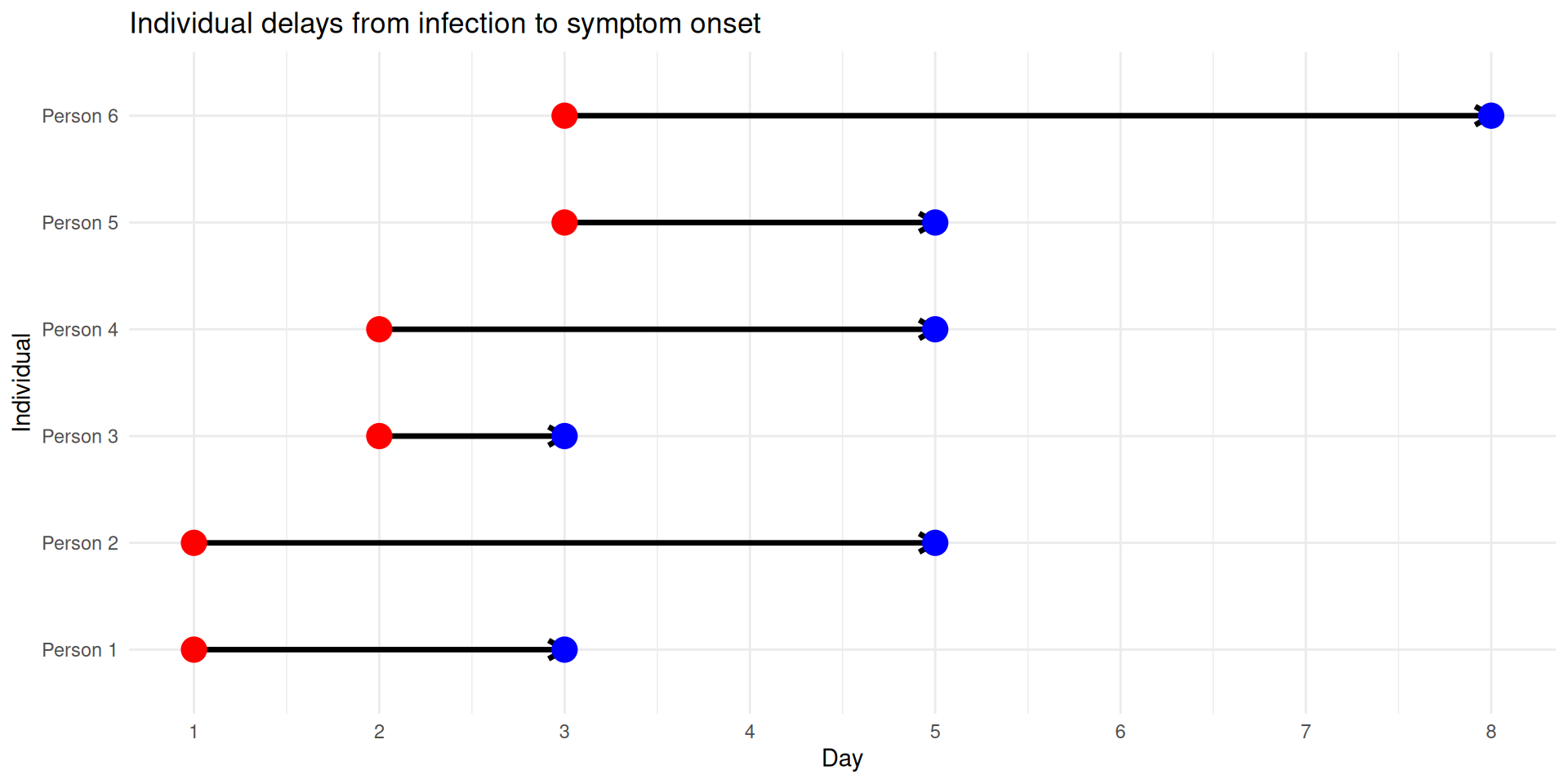
Individual delay distributions
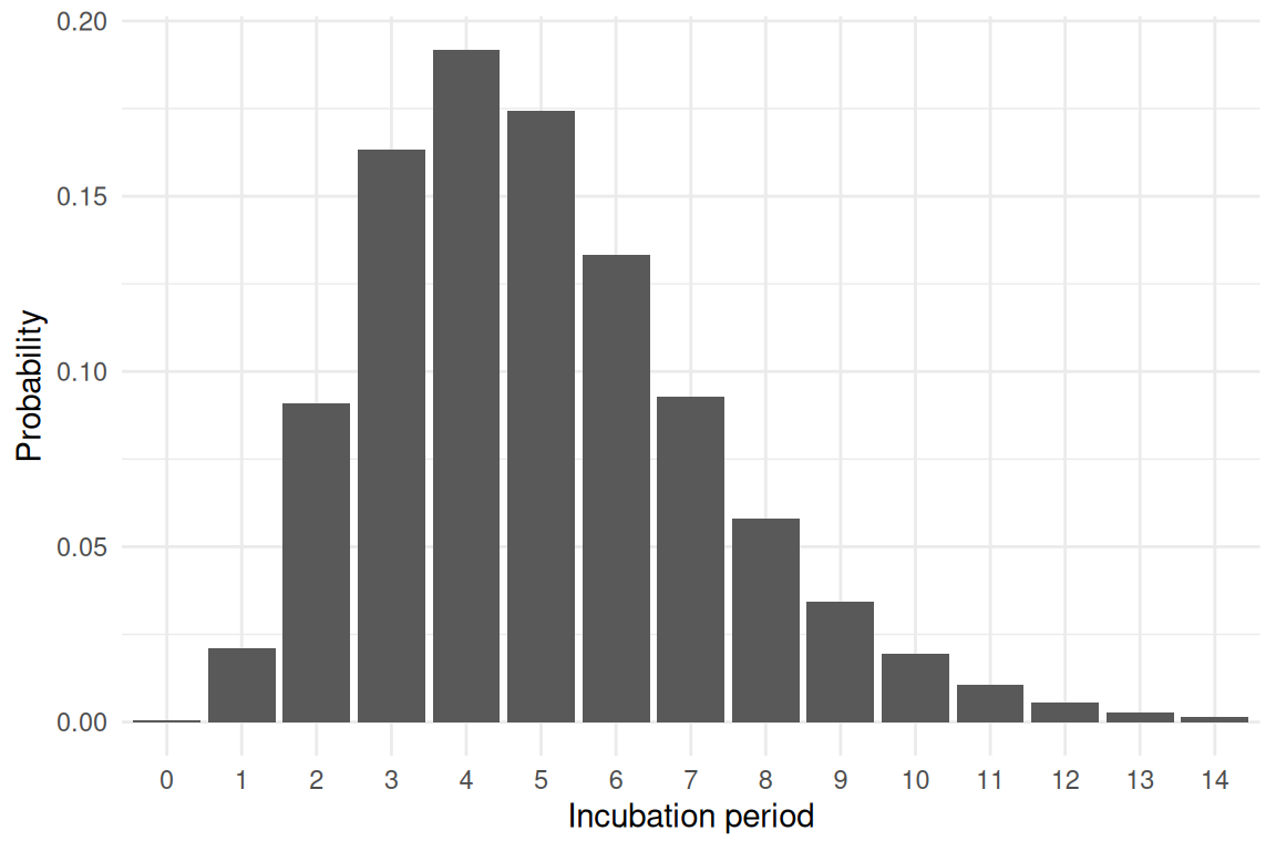
Let us consider an epidemiological process that is characterised by a discrete distribution \(f_d\).
Example:
\(f_d\): Probability of having incubation period of \(d\) days.
Individual to population: A simple example
If we know individual events, we can add a draw from the delay distribution and sum up the resulting delays.
Why not use individual delays?
- we don’t always have individual data available
- we often model other processes at the population level (such as transmission) and so being able to model delays on the same scale is useful
- doing the computation at the population level requires fewer calculations (i.e. is faster)
- however, a downside is that we won’t have realistic uncertainty, especially if the number of individuals is small
Convolution: From individual to population
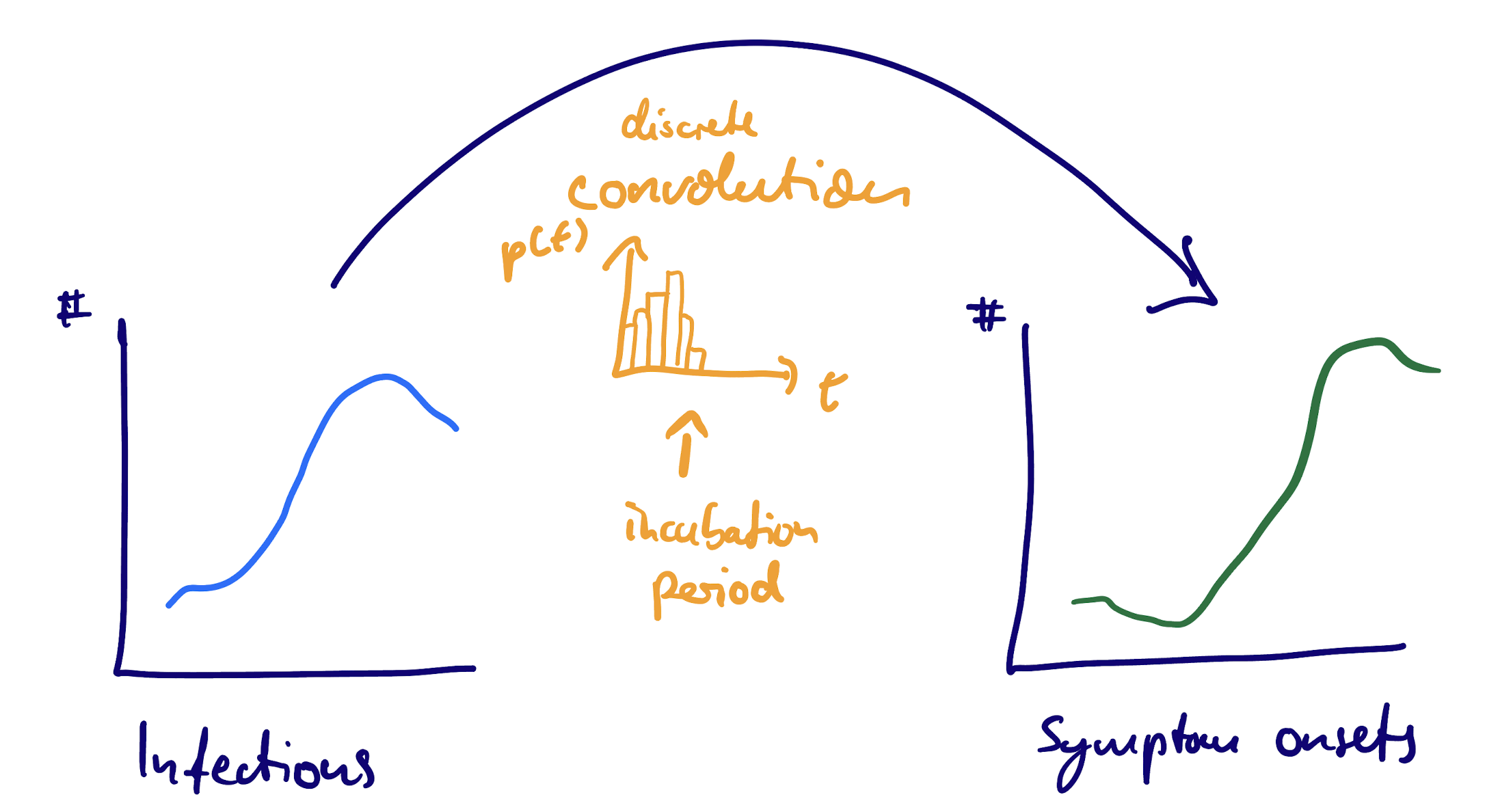
Population level counts: The mathematics
If the number of individuals \(P_{t'}\) that have their primary event at time \(t'\) then we can rewrite this as
\[ S_t = \sum_{t'} P_{t'} f_{t - t'} \]
This operation is called a (discrete) convolution of \(P\) with \(f_d\).
We can use convolutions with the delay distribution that applies at the individual level to determine population-level counts.
What if \(f\) is continuous?
Having moved to the population level, we can’t estimate individual-level event times any more.
Instead, we discretise the distribution (remembering that it is double censored - as both events are censored).
This can be solved mathematically but in the session we will use simulation.
Your Turn
- Simulate convolutions with infection counts
- Discretise continuous distributions
- Estimate parameters numbers of infections from number of symptom onsets, using a convolution model
Delay distributions at the population level