functions {
  #include "functions/convolve_with_delay.stan"
}

data {
  int n;            // number of time days
  array[n] int obs; // observed onsets
  int<lower = 1> ip_max; // max incubation period
  // probability mass function of incubation period distribution (first index zero)
  array[ip_max + 1] real ip_pmf;
}

parameters {
  array[n] real<lower = 0> infections;
}

transformed parameters {
  array[n] real onsets = convolve_with_delay(infections, ip_pmf);
}

model {
  // priors
  infections ~ normal(0, 10) T[0, ];
  obs ~ poisson(onsets);
}Introduction to the time-varying reproduction number
Nowcasting and forecasting of infectious disease dynamics
Convolution session
Prior for infections at time \(t\) is independent from infections at all other time points. Is this reasonable?
What if we convolve infections with infections?
We can extend the convolution concept from the last session:
- Previous session: infections → symptoms (via incubation period)
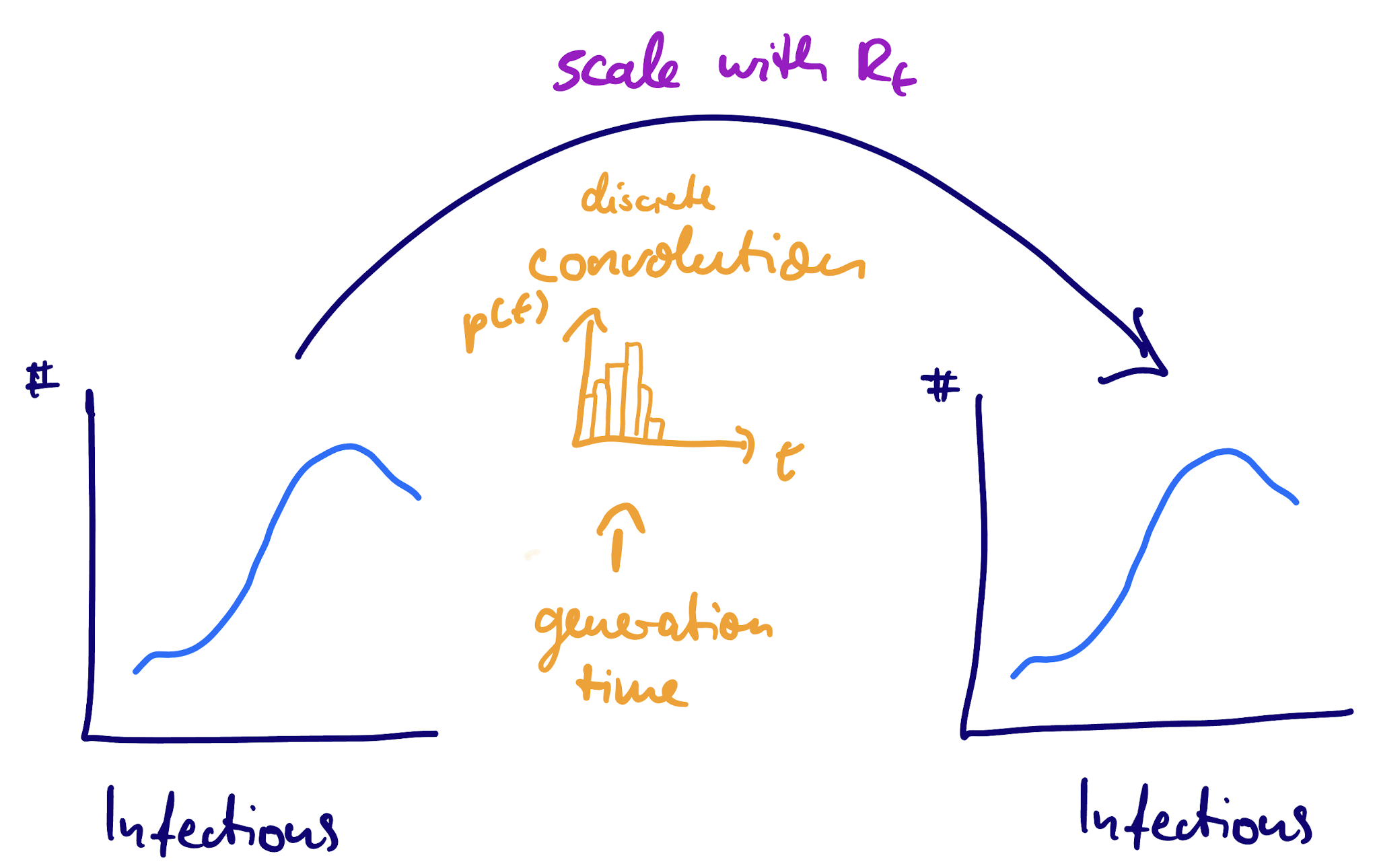
- This session: infections → infections (via generation time)
Generation time: infection to infection
Here rather than the time from infection (person A) to symptoms (person B, infected by A) we have the time from infection (person A) to infection (person B, infected by A).
This is known as the generation time distribution (\(g(t)\)).
Generation time: notation
We can write the convolution as:
\[ I_t = \mathrm{scaling} \times \sum_{t' < t} I_t' g(t - t') \]
However, unlike the infection to symptoms case here we don’t assume that the two time series have the same magnitude so need to introduce a scaling.
What is this scaling?
The renewal equation as a convolution
The scaling factor: reproduction number
Let’s assume we have \(I_0\) infections at time 0, and the scaling doesn’t change in time.
How many people will they go on to infect?
\[ I = \mathrm{scaling} \times \sum_{t=0}^\infty I_0 g(t) = \mathrm{scaling} * I_0 \]
The scaling can be interpreted as the reproduction number \(R_0\) (assuming a susceptible population).
The renewal equation
If \(R_t\) can change over time, it can be interpreted as the (“instantaneous”) reproduction number:
\[ I_t = R_t \times \sum_{t' < t} I_t' g(t - t') \]
We can estimate \(R_t\) from a time series of infections using the renewal equation.
Your Turn
- Simulate infections using the renewal equation
- Estimate reproduction numbers using a time series of infections
- Combine with delay distributions to jointly infer infections and R from a time series of outcomes
Introduction to the time-varying reproduction number