Forecast ensembles

Introduction

As we saw in the session on different forecasting models, different modelling approaches have different strength and weaknesses, and we do not usually know in advance which one will produce the best forecast in any given situation. We can classify models along a spectrum by how much they include an understanding of underlying processes, or mechanisms; or whether they emphasise drawing from the data using a statistical approach. One way to attempt to draw strength from a diversity of approaches is the creation of so-called forecast ensembles from the forecasts produced by different models.

In this session, we’ll start with forecasts from the models we explored in the forecasting models session and build ensembles of these models. We will then compare the performance of these ensembles to the individual models and to each other.

Representations of probabilistic forecasts

Probabilistic predictions can be described as coming from a probabilistic probability distributions. In general and when using complex models such as the one we discuss in this course, these distributions can not be expressed in a simple analytical formal as we can do if, e.g. talking about common probability distributions such as the normal or gamma distributions. Instead, we typically use a limited number of samples generated from Monte-Carlo methods to represent the predictive distribution. However, this is not the only way to characterise distributions.

A quantile is the value that corresponds to a given quantile level of a distribution. For example, the median is the 50th quantile of a distribution, meaning that 50% of the values in the distribution are less than the median and 50% are greater. Similarly, the 90th quantile is the value that corresponds to 90% of the distribution being less than this value. If we characterise a predictive distribution by its quantiles, we specify these values at a range of specific quantile levels, e.g. from 5% to 95% in 5% steps.

Deciding how to represent forecasts depends on many things, for example the method used (and whether it produces samples by default) but also logistic considerations. Many collaborative forecasting projects and so-called forecasting hubs use quantile-based representations of forecasts in the hope to be able to characterise both the centre and tails of the distributions more reliably and with less demand on storage space than a sample-based representation.

Slides

• Introduction to ensembles

Objectives

The aim of this session is to introduce the concept of ensembles of forecasts and to evaluate the performance of ensembles of the models we explored in the forecasting models session.

Setup

Source file

The source file of this session is located at sessions/forecast-ensembles.qmd.

Libraries used

In this session we will use the nfidd package to load a data set of infection times and access stan models and helper functions, the dplyr and tidyr packages for data wrangling, ggplot2 library for plotting, the tidybayes package for extracting results of the inference and the scoringutils package for evaluating forecasts. We will also use qrensemble for quantile regression averaging and lopensemble for mixture ensembles (also called linear opinion pool).

library("nfidd")
library("dplyr")
library("tidyr")
library("ggplot2")
library("scoringutils")
library("qrensemble")
library("lopensemble")

Tip

The best way to interact with the material is via the Visual Editor of RStudio.

Initialisation

We set a random seed for reproducibility. Setting this ensures that you should get exactly the same results on your computer as we do.

set.seed(123)

Individual forecast models

In this session we will use the forecasts from the models we explored in the session on forecasting models. There all shared the same basic renewal with delays structure but used different models for the evolution of the effective reproduction number over time. These were:

• A random walk model
• A differenced autoregressive model referred to as “More statistical”
• A simple model of susceptible depletion referred to as “More mechanistic”

For the purposes of this session the precise details of the models are not critical to the concepts we are exploring.

As in the session on forecast evaluation, we have fitted these models to a range of forecast dates so you don’t have to wait for the models to fit.

data(rw_forecasts, stat_forecasts, mech_forecasts)
forecasts <- bind_rows(
  rw_forecasts,
  mutate(stat_forecasts, model = "More statistical"),
  mutate(mech_forecasts, model = "More mechanistic")
)

forecasts

# A tibble: 672,000 × 7
     day .draw .variable .value horizon origin_day model      
   <dbl> <int> <chr>      <dbl>   <int>      <dbl> <chr>      
 1    23     1 forecast       9       1         22 Random walk
 2    23     2 forecast       5       1         22 Random walk
 3    23     3 forecast       5       1         22 Random walk
 4    23     4 forecast       3       1         22 Random walk
 5    23     5 forecast       5       1         22 Random walk
 6    23     6 forecast       6       1         22 Random walk
 7    23     7 forecast       3       1         22 Random walk
 8    23     8 forecast       2       1         22 Random walk
 9    23     9 forecast       2       1         22 Random walk
10    23    10 forecast       4       1         22 Random walk
# ℹ 671,990 more rows

How did we generate these forecasts?

We generated these forecasts using the code in data-raw/generate-example-forecasts.r which uses the same approach we just took before for a single forecast date but generalises it to many forecast dates.

Some important things to note about these forecasts:

• We used a 14 day forecast horizon.
• Each forecast used all the data up to the forecast date.
• We generated 1000 predictive posterior samples for each forecast.
• We started forecasting 3 weeks into the outbreak and then forecast every 7 days until the end of the data (excluding the last 14 days to allow a full forecast).
• We use the same simulated outbreak data as before:

gen_time_pmf <- make_gen_time_pmf()
ip_pmf <- make_ip_pmf()
onset_df <- simulate_onsets(
  make_daily_infections(infection_times), gen_time_pmf, ip_pmf
)
head(onset_df)

# A tibble: 6 × 3
    day onsets infections
  <dbl>  <int>      <int>
1     1      0          0
2     2      0          1
3     3      0          0
4     4      1          2
5     5      0          1
6     6      0          1

Forecast ensembles

We will now move to creating forecasts as a combination of multiple forecasts. This procedure is also sometimes called stacking, and the resulting forecasts are said to come from ensembles of forecast models.

Quantile-based ensembles

We will first consider forecasts based on the individual quantiles of each model. This corresponds to a situation where each forecast aims to correctly determine a single target predictive distribution. By taking an average of all models, we aim to get a better estimate of this distribution than from the individual models. If we have reason to believe that some models are better than others at estimating this distribution, we can create a weighted version of this average.

Converting sample-based forecasts to quantile-based forecasts

As in this session we will be thinking about forecasts in terms quantiles of the predictive distributions, we will need to convert our sample based forecasts to quantile-based forecasts. We will do this by focusing at the marginal distribution at each predicted time point, that is we treat each time point as independent of all others and calculate quantiles based on the sample predictive trajectories at that time point. An easy way to do this is to use the {scoringutils} package. The steps to do this are to first declare the forecasts as sample forecasts.

sample_forecasts <- forecasts |>
  left_join(onset_df, by = "day") |>
  filter(!is.na(.value)) |>
  as_forecast_sample(
    forecast_unit = c("origin_day", "horizon", "model", "day"),
    observed = "onsets",
    predicted = ".value",
    sample_id = ".draw"
  )
sample_forecasts

Forecast type: sample

Forecast unit:

origin_day, horizon, model, and day

        sample_id predicted observed origin_day horizon            model   day
            <int>     <num>    <int>      <num>   <int>           <char> <num>
     1:         1         9        4         22       1      Random walk    23
     2:         2         5        4         22       1      Random walk    23
     3:         3         5        4         22       1      Random walk    23
     4:         4         3        4         22       1      Random walk    23
     5:         5         5        4         22       1      Random walk    23
    ---                                                                       
671996:       996         4        2        127      14 More mechanistic   141
671997:       997         2        2        127      14 More mechanistic   141
671998:       998         1        2        127      14 More mechanistic   141
671999:       999         2        2        127      14 More mechanistic   141
672000:      1000         1        2        127      14 More mechanistic   141

and then convert to quantile forecasts.

quantile_forecasts <- sample_forecasts |>
  as_forecast_quantile()
quantile_forecasts

Forecast type: quantile

Forecast unit:

origin_day, horizon, model, and day

      observed origin_day horizon            model   day quantile_level
         <int>      <num>   <int>           <char> <num>          <num>
   1:        4         22       1      Random walk    23           0.05
   2:        4         22       1      Random walk    23           0.25
   3:        4         22       1      Random walk    23           0.50
   4:        4         22       1      Random walk    23           0.75
   5:        4         22       1      Random walk    23           0.95
  ---                                                                  
3356:        2        127      14 More mechanistic   141           0.05
3357:        2        127      14 More mechanistic   141           0.25
3358:        2        127      14 More mechanistic   141           0.50
3359:        2        127      14 More mechanistic   141           0.75
3360:        2        127      14 More mechanistic   141           0.95
      predicted
          <num>
   1:         1
   2:         2
   3:         3
   4:         5
   5:         8
  ---          
3356:         0
3357:         2
3358:         3
3359:         4
3360:         6

What is happening here?

• Internally scoringutils is calculating the quantiles of the sample-based forecasts.
• It does this by using a set of default quantiles but different ones can be specified by the user to override the default.
• It then calls the quantile() function from base R to calculate the quantiles.
• This is estimating the value that corresponds to each given quantile level by ordering the samples and then taking the value at the appropriate position.

Simple unweighted ensembles

A good place to start when building ensembles is to take the mean or median of the unweighted forecast at each quantile level, and treat these as quantiles of the ensemble predictive distribution. Typically, the median is preferred when outlier forecasts are likely to be present as it is less sensitive to these. However, the mean is preferred when forecasters have more faith in models that diverge from the median performance and want to represent this in the ensemble.

Vincent average

The procedure of calculating quantiles of a new distribution as a weighted average of quantiles of constituent distributions (e.g., different measurements) is called a Vincent average, after the biologist Stella Vincent who described this as early as 1912 when studying the function of whiskers in the behaviour of white rats.

Construction

We can calculate the mean quantile ensemble by taking the mean of the forecasts at each quantile level.

mean_ensemble <- quantile_forecasts |>
  as_tibble() |>
  summarise(
    predicted = mean(predicted),
    observed = unique(observed),
    model = "Mean ensemble",
    .by = c(origin_day, horizon, quantile_level, day)
  )

Similarly, we can calculate the median ensemble by taking the median of the forecasts at each quantile level.

median_ensemble <- quantile_forecasts |>
  as_tibble() |>
  summarise(
    predicted = median(predicted),
    observed = unique(observed),
    model = "Median ensemble",
    .by = c(origin_day, horizon, quantile_level, day)
  )

We combine the ensembles into a single data frame along with the individual forecasts in order to make visualisation easier.

simple_ensembles <- bind_rows(
  mean_ensemble,
  median_ensemble,
  quantile_forecasts
)

Visualisation

How do these ensembles visually differ from the individual models? Lets start by plotting a single forecast from each model and comparing them.

plot_ensembles <- function(data, obs_data) {
  data |>
    pivot_wider(names_from = quantile_level, values_from = predicted) |>
    ggplot(aes(x = day)) +
    geom_ribbon(
    aes(
      ymin = .data[["0.05"]], ymax = .data[["0.95"]], fill = model,
        group = origin_day
      ),
      alpha = 0.2
    ) +
    geom_ribbon(
      aes(
        ymin = .data[["0.25"]], ymax = .data[["0.75"]], fill = model,
        group = origin_day
      ),
      alpha = 0.5
    ) +
    geom_point(
      data = obs_data,
      aes(x = day, y = onsets), color = "black"
    ) +
    scale_color_binned(type = "viridis") +
    facet_wrap(~model) +
    theme(legend.position = "none")
}

plot_single_forecasts <- simple_ensembles |>
  filter(origin_day == 57) |>
  plot_ensembles(onset_df |> filter(day >= 57, day <= 57 + 14))

plot_single_forecasts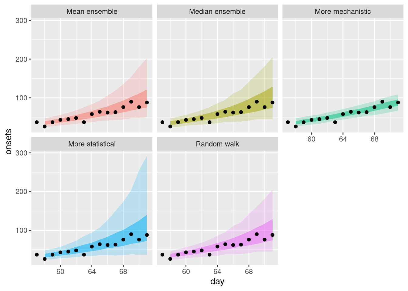

Again we can get a different perspective by plotting the forecasts on the log scale.

plot_single_forecasts +
  scale_y_log10()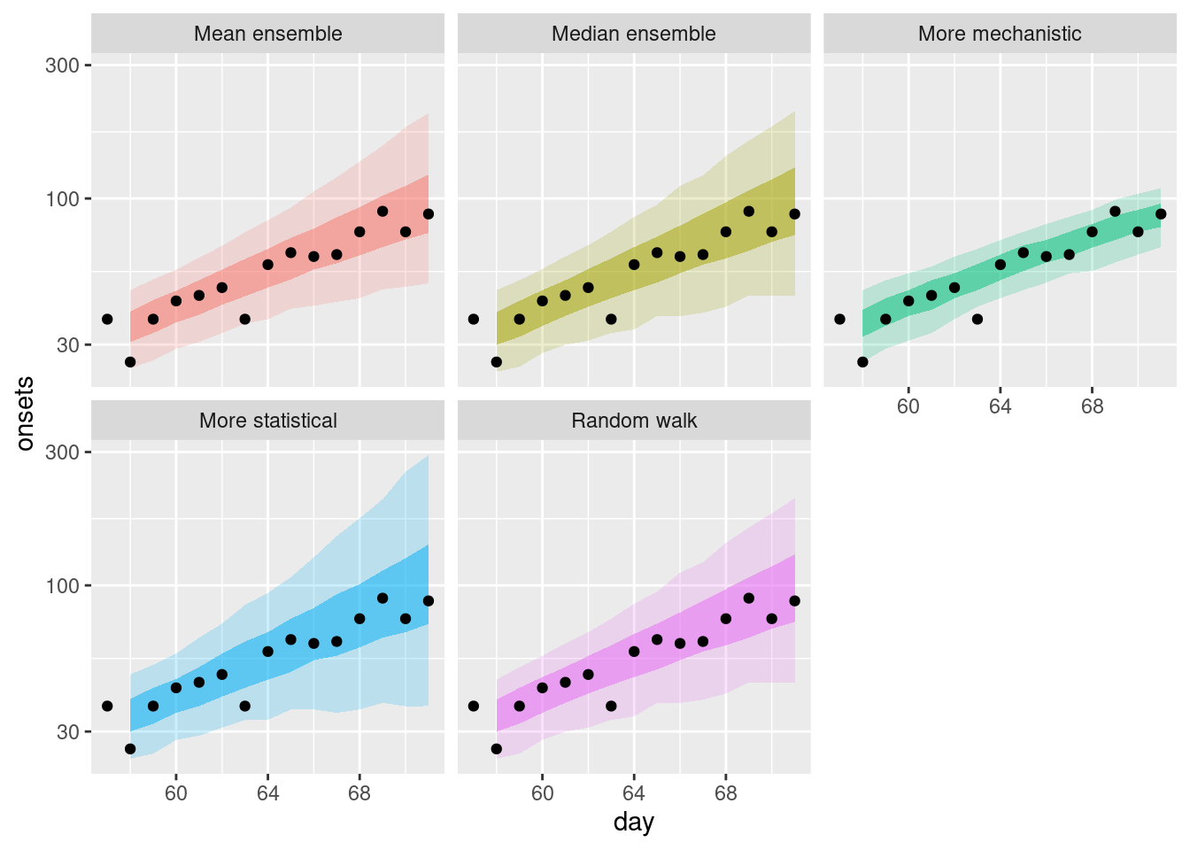

Take 2 minutes

How do these ensembles compare to the individual models? How do they differ from each other?

Solution

How do these ensembles compare to the individual models?

• Both of the simple ensembles appear to be less variable than the statistical models but are more variable than the mechanistic model.
• Both ensembles are more like the statistical models than the mechanistic model.

How do they differ from each other?

• The mean ensemble has slightly tighter uncertainty bounds than the median ensemble.

Now lets plot a range of forecasts from each model and ensemble.

plot_multiple_forecasts <- simple_ensembles |>
  plot_ensembles(onset_df |> filter(day >= 21)) +
  lims(y = c(0, 400))

plot_multiple_forecasts

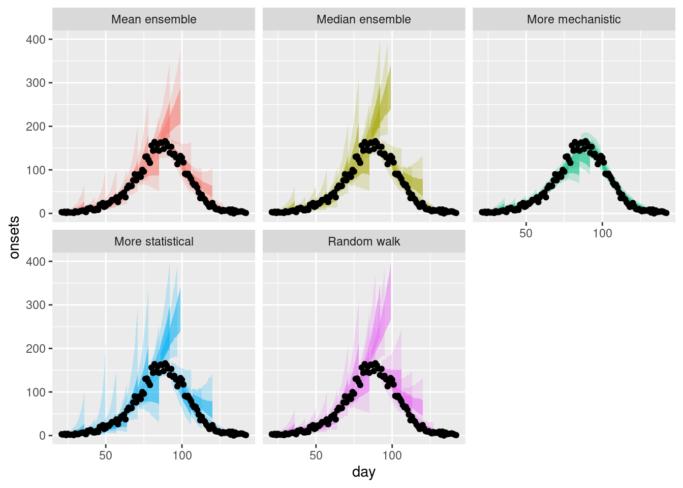
Again we can get a different perspective by plotting the forecasts on the log scale.

plot_multiple_forecasts +
  scale_y_log10()

Scale for y is already present.
Adding another scale for y, which will replace the existing scale.

Warning in scale_y_log10(): log-10 transformation introduced infinite values.
log-10 transformation introduced infinite values.
log-10 transformation introduced infinite values.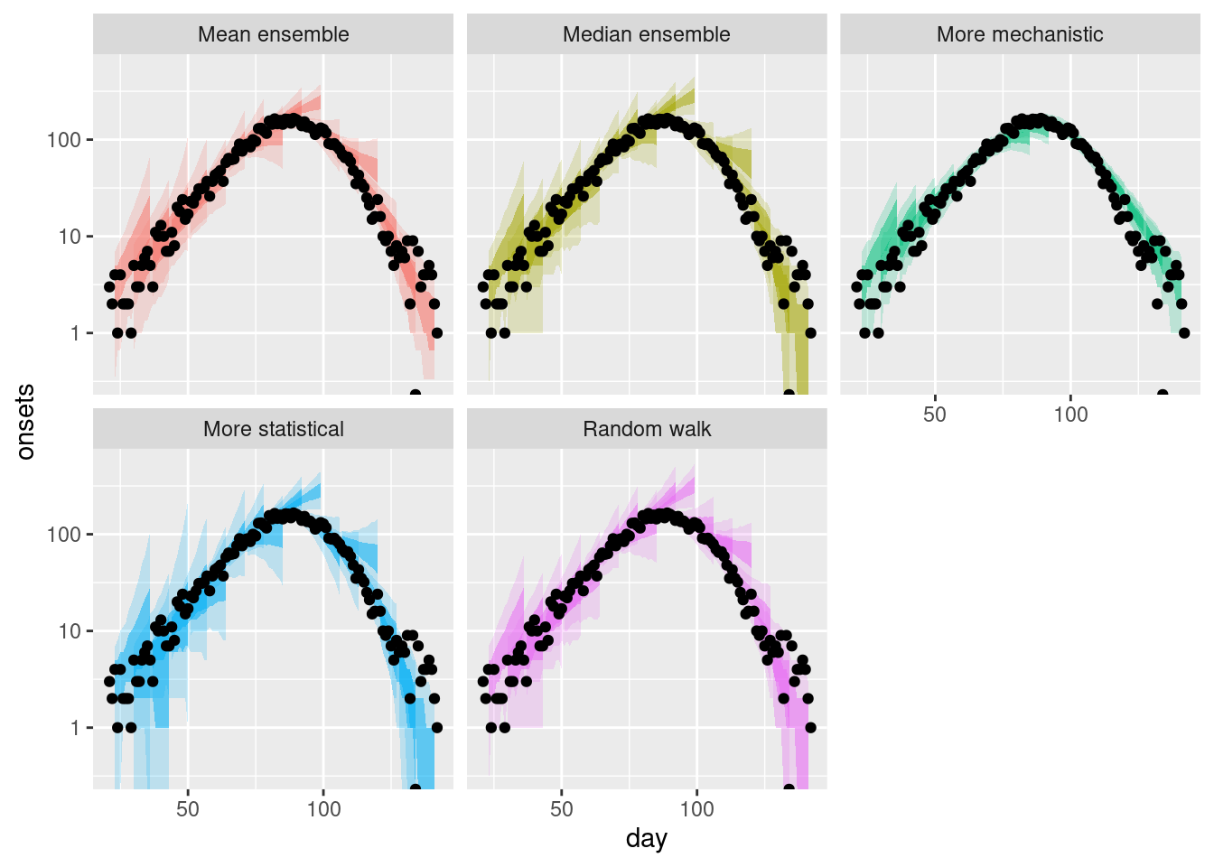

Take 2 minutes

How do these ensembles compare to the individual models?

How do they differ from each other?

Are there any differences across forecast dates?

Solution

How do these ensembles compare to the individual models?

• As before, the ensembles appear to be less variable than the statistical models but more variable than the mechanistic model.

How do they differ from each other?

• The mean ensemble has marginally tighter uncertainty bounds than the median ensemble as for the single forecast.

Are there any differences across forecast dates?

• The mean ensemble appears to be more variable across forecast dates than the median ensemble with this being more pronounced after the peak of the outbreak.

Evaluation

As in the forecast evaluation session, we can evaluate the accuracy of the ensembles using the {scoringutils} package and in particular the score() function.

ensemble_scores <- simple_ensembles |>
  as_forecast_quantile(forecast_unit = c("origin_day", "horizon", "model")) |>
  score()

Note

The weighted interval score (WIS) is a proper scoring rule for quantile forecasts that approximates the Continuous Ranked Probability Score (CRPS) by considering a weighted sum of multiple prediction intervals. As the number of intervals increases, the WIS converges to the CRPS, combining sharpness and penalties for over- and under-prediction.

We see it here as we are scoring quantiles and not samples hence we cannot use CRPS as we did before.

Again we start with a high level overview of the scores by model.

ensemble_scores |>
  summarise_scores(by = c("model"))

              model       wis overprediction underprediction dispersion
             <char>     <num>          <num>           <num>      <num>
1:    Mean ensemble  8.368094       4.053482       1.1252976   3.189314
2:  Median ensemble 10.408312       5.707768       1.2781250   3.422420
3:      Random walk 11.942152       7.041786       0.8459821   4.054384
4: More statistical 11.036451       5.458304       1.7772321   3.800915
5: More mechanistic  5.647196       1.664643       2.2699107   1.712643
          bias interval_coverage_50 interval_coverage_90 ae_median
         <num>                <num>                <num>     <num>
1:  0.18348214            0.5089286            0.8750000  12.80208
2:  0.13883929            0.5178571            0.8660714  15.92857
3:  0.20133929            0.5133929            0.8616071  18.25893
4: -0.02857143            0.5000000            0.8526786  16.83482
5:  0.21741071            0.4598214            0.7633929   8.75000

Take 5 minutes

What do you think the scores are telling you? Which model do you think is best? What other scoring breakdowns might you want to look at?

Solution

What do you think the scores are telling you? Which model do you think is best?

• The mean ensemble appears to be the best performing ensemble model overall.
• However, the more mechanistic model appears to be the best performing model overall.

What other scoring breakdowns might you want to look at?

• There might be variation over forecast dates or horizons between the different ensemble methods

Unweighted ensembles of filtered models

A simple method that is often used to improve ensemble performance is to prune out models that perform very poorly. Balancing this can be tricky however as it can be hard to know how much to prune. The key tradeoff to consider is how much to optimise for which models have performed well in the past (and what your definition of the past is, for example all time or only the last few weeks) versus how much you want to allow for the possibility that these models may not perform well in the future.

Construction

As we just saw, the random walk model (our original baseline model) is performing poorly in comparison to the other models. We can remove this model from the ensemble and see if this improves the performance of the ensemble.

Warning

Here we are technically cheating a little as we are using the test data to help select the models to include in the ensemble. In the real world you would not do this as you would not have access to the test data and so this is an idealised scenario.

filtered_models <- quantile_forecasts |>
  filter(model != "Random walk")

We then need to recalculate the ensembles. First the mean ensemble,

filtered_mean_ensembles <- filtered_models |>
  as_tibble() |>
  summarise(
    predicted = mean(predicted),
    observed = unique(observed),
    model = "Mean filtered ensemble",
    .by = c(origin_day, horizon, quantile_level, day)
  )

and then the median ensemble.

filtered_median_ensembles <- filtered_models |>
  as_tibble() |>
  summarise(
    predicted = median(predicted),
    observed = unique(observed),
    model = "Median filtered ensemble",
    .by = c(origin_day, horizon, quantile_level, day)
  )

We combine these new ensembles with our previous ensembles in order to make visualisation easier.

filtered_ensembles <- bind_rows(
  filtered_mean_ensembles,
  filtered_median_ensembles,
  simple_ensembles
)

Visualisation

As for the simple ensembles, we can plot a single forecast from each model and ensemble.

filtered_ensembles |>
  filter(origin_day == 57) |>
  plot_ensembles(onset_df |> filter(day >= 57, day <= 57 + 14))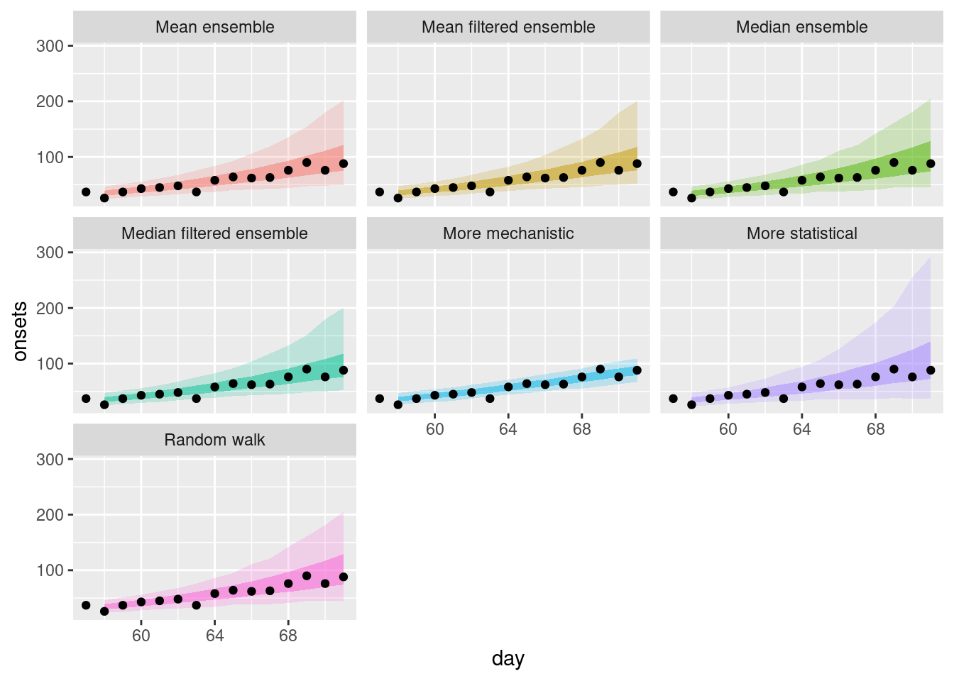

and on the log scale.

filtered_ensembles |>
  filter(origin_day == 57) |>
  plot_ensembles(onset_df |> filter(day >= 57, day <= 57 + 14)) +
  scale_y_log10()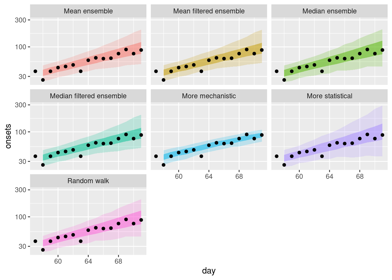

To get an overview we also plot a range of forecasts from each model and ensemble.

plot_multiple_filtered_forecasts <- filtered_ensembles |>
  plot_ensembles(onset_df |> filter(day >= 21)) +
  lims(y = c(0, 400))
plot_multiple_filtered_forecasts

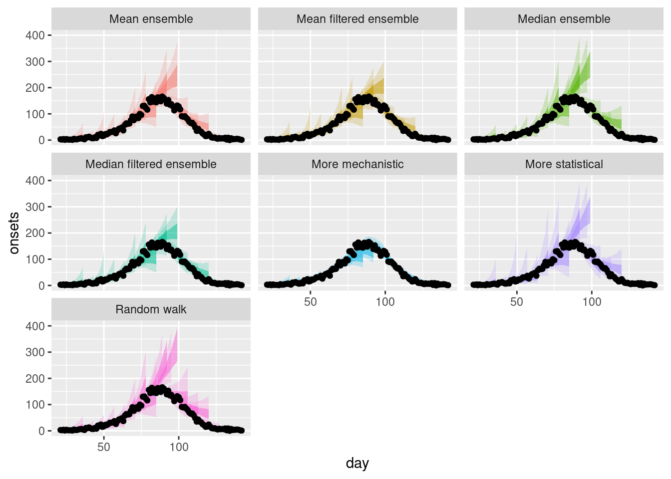
and on the log scale.

plot_multiple_filtered_forecasts +
  scale_y_log10()

Scale for y is already present.
Adding another scale for y, which will replace the existing scale.

Warning in scale_y_log10(): log-10 transformation introduced infinite values.
log-10 transformation introduced infinite values.
log-10 transformation introduced infinite values.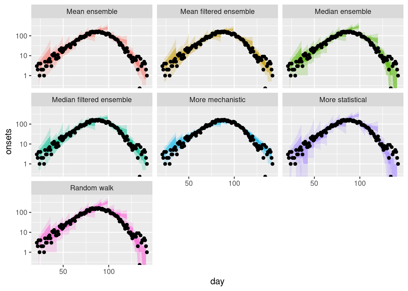

Take 2 minutes

How do the filtered ensembles compare to the simple ensembles? Which do you think is best?

Solution

How do the filtered ensembles compare to the simple ensembles?

• The filtered ensembles appear to be less variable than the simple ensembles.
• The filtered ensembles appear to be more like the mechanistic model than the simple ensembles.

Which do you think is best?

• Visually, the filtered ensembles appear very similar. This makes sense given we know there are only two models left in the ensemble.

Evaluation

Let us score the filtered ensembles.

filtered_ensemble_scores <- filtered_ensembles |>
  as_forecast_quantile(
    forecast_unit = c(
      "origin_day", "horizon", "model"
    )
  ) |>
  score()

Again we can get a high level overview of the scores by model.

filtered_ensemble_scores |>
  summarise_scores(by = c("model"))

                      model       wis overprediction underprediction dispersion
                     <char>     <num>          <num>           <num>      <num>
1:   Mean filtered ensemble  7.001690       2.785045       1.4598661   2.756779
2: Median filtered ensemble  7.001690       2.785045       1.4598661   2.756779
3:            Mean ensemble  8.368094       4.053482       1.1252976   3.189314
4:          Median ensemble 10.408312       5.707768       1.2781250   3.422420
5:              Random walk 11.942152       7.041786       0.8459821   4.054384
6:         More statistical 11.036451       5.458304       1.7772321   3.800915
7:         More mechanistic  5.647196       1.664643       2.2699107   1.712643
          bias interval_coverage_50 interval_coverage_90 ae_median
         <num>                <num>                <num>     <num>
1:  0.13482143            0.5089286            0.8705357  10.76562
2:  0.13482143            0.5089286            0.8705357  10.76562
3:  0.18348214            0.5089286            0.8750000  12.80208
4:  0.13883929            0.5178571            0.8660714  15.92857
5:  0.20133929            0.5133929            0.8616071  18.25893
6: -0.02857143            0.5000000            0.8526786  16.83482
7:  0.21741071            0.4598214            0.7633929   8.75000

Take 2 minutes

How do the filtered ensembles compare to the simple ensembles?

Solution

How do the filtered ensembles compare to the simple ensembles?

• The filtered ensembles appear to be more accurate than the simple ensembles.
• As you would expect they are an average of the more mechanistic model and the more statistical model.
• As there are only two models in the ensemble, the median and mean ensembles are identical.
• For the first time there are features of the ensemble that outperform the more mechanistic model though it remains the best performing model overall.

Weighted ensembles

The simple mean and median we used to average quantiles earlier treats every model as the same. We could try to improve performance by replacing this with a weighted mean (or weighted median), for example given greater weight to models that have proven to make better forecasts. Here we will explore two common weighting methods based on quantile averaging:

• Inverse WIS weighting
• Quantile regression averaging

Inverse WIS weighting is a simple method that weights the forecasts by the inverse of their WIS over some period (note that identifying what this period should be in order to produce the best forecasts is not straightforward as predictive performance may vary over time if models are good at different things). The main benefit of WIS weighting over other methods is that it is simple to understand and implement. However, it does not optimise the weights directly to produce the best forecasts. It relies on the hope that giving more weight to better performing models yields a better ensemble

Quantile regression averaging (QRA), on the other hand, optimises the weights directly in order to yield the best scores on past data.

Construction

Inverse WIS weighting

In order to perform inverse WIS weighting we first need to calculate the WIS for each model. We already have this from the previous evaluation so we can reuse this.

model_scores <- quantile_forecasts |>
  score()
cumulative_scores <- list()
## filter for scores up to the origin day of the forecast
for (day_by in unique(model_scores$origin_day)) {
  cumulative_scores[[as.character(day_by)]] <- model_scores |>
    filter(origin_day < day_by) |>
    summarise_scores(by = "model") |>
    mutate(day_by = day_by)
}
weights_per_model <- bind_rows(cumulative_scores) |>
  select(model, day_by, wis) |>
  mutate(inv_wis = 1 / wis) |>
  mutate(
    inv_wis_total_by_date = sum(inv_wis), .by = day_by
  ) |>
  mutate(weight = inv_wis / inv_wis_total_by_date) |> ## normalise
  select(model, origin_day = day_by, weight)

weights_per_model |>
  pivot_wider(names_from = model, values_from = weight)

# A tibble: 15 × 4
   origin_day `Random walk` `More statistical` `More mechanistic`
        <dbl>         <dbl>              <dbl>              <dbl>
 1         29         0.325              0.412              0.262
 2         36         0.363              0.381              0.256
 3         43         0.370              0.353              0.277
 4         50         0.362              0.324              0.314
 5         57         0.345              0.302              0.353
 6         64         0.329              0.293              0.379
 7         71         0.308              0.285              0.406
 8         78         0.354              0.292              0.354
 9         85         0.316              0.306              0.378
10         92         0.239              0.250              0.511
11         99         0.239              0.251              0.510
12        106         0.237              0.254              0.509
13        113         0.228              0.246              0.526
14        120         0.233              0.254              0.513
15        127         0.237              0.258              0.505

Now lets apply the weights to the forecast models. As we can only use information that was available at the time of the forecast to perform the weighting, we use weights from two weeks prior to the forecast date to inform each ensemble.

inverse_wis_ensemble <- quantile_forecasts |>
  as_tibble() |>
  left_join(
    weights_per_model |>
      mutate(origin_day = origin_day + 14),
    by = c("model", "origin_day")
  ) |>
  # assign equal weights if no weights are available
  mutate(weight = ifelse(is.na(weight), 1/3, weight)) |>
  summarise(
    predicted = sum(predicted * weight),
    observed = unique(observed),
    model = "Inverse WIS ensemble",
    .by = c(origin_day, horizon, quantile_level, day)
  )

Quantile regression averaging

We futher to perform quantile regression averaging (QRA) for each forecast date. Again we need to consider how many previous forecasts we wish to use to inform each ensemble forecast. Here we decide to use up to 3 weeks of previous forecasts to inform each QRA ensemble. We use the qrensemble package to perform this task.

forecast_dates <- quantile_forecasts |>
  as_tibble() |>
  pull(origin_day) |>
  unique()

qra_by_forecast <- function(
  quantile_forecasts,
  forecast_dates,
  group = c("target_end_date"), 
  ...
) {
  lapply(forecast_dates, \(x) {
    quantile_forecasts |>
      mutate(target_end_date = x) |>
      dplyr::filter(origin_day <= x) |>
      dplyr::filter(origin_day >= x - (3 * 7 + 1)) |>
      dplyr::filter(origin_day == x | day <= x) |>
      qra(
        group = group,
        target = c(origin_day = x),
        ...
      )
  })
}

qra_ensembles_obj <- qra_by_forecast(
  quantile_forecasts,
  forecast_dates[-1],
  group = c("target_end_date")
)

qra_weights <- seq_along(qra_ensembles_obj) |>
  lapply(\(i) attr(qra_ensembles_obj[[i]], "weights") |>
    mutate(origin_day = forecast_dates[i + 1])
  ) |>
  bind_rows() |>
  dplyr::filter(quantile == 0.5) |>
  select(-quantile)

qra_ensembles <- qra_ensembles_obj |>
  bind_rows()

Instead of creating a single optimised ensemble and using this for all forecast horizons we might also want to consider a separate optimised QRA ensemble for each forecast horizon, reflecting that models might perform differently depending on how far ahead a forecast is produced. We can do this using qra() with the group argument.

qra_ensembles_by_horizon <- qra_by_forecast(
  quantile_forecasts,
  forecast_dates[-c(1:2)],
  group = c("horizon", "target_end_date"),
  model = "QRA by horizon"
)

qra_weights_by_horizon <- seq_along(qra_ensembles_by_horizon) |>
  lapply(\(i) attr(qra_ensembles_by_horizon[[i]], "weights") |>
    mutate(origin_day = forecast_dates[i + 2])
  ) |>
  bind_rows()

Sample-based weighted ensembles

Quantile averaging can be interpreted as a combination of different uncertain estimates of a true distribution of a given shape. Instead, we might want to interpret multiple models as multiple possible versions of this truth, with weights assigned to each of them representing the probability of each one being the true one. In that case, we want to create a (weighted) mixture distribution of the constituent models. This can be done from samples, with weights tuned to optimise the CRPS. The procedure is also called a linear opinion pool. Once again one can create unweighted, filtered unweighted and weighted ensembles. For now we will just consider weighted ensembles. We use the lopensemble package to perform this task.

## lopensemble expects a "date" column indicating the timing of forecasts
lop_forecasts <- sample_forecasts |>
  rename(date = day)

lop_by_forecast <- function(
  sample_forecasts,
  forecast_dates,
  group = c("target_end_date"),
  ...
) {
  lapply(forecast_dates, \(x) {
    y <- sample_forecasts |>
      mutate(target_end_date = x) |>
      dplyr::filter(origin_day <= x) |>
      dplyr::filter(origin_day >= x - (3 * 7 + 1)) |>
      dplyr::filter(origin_day == x | date <= x)
    lop <- mixture_from_samples(y) |>
      filter(date > x) |>
      mutate(origin_day = x)
    return(lop)
  })
}

lop_ensembles_obj <- lop_by_forecast(
  lop_forecasts,
  forecast_dates[-1]
)

lop_weights <- seq_along(lop_ensembles_obj) |>
  lapply(\(i) attr(lop_ensembles_obj[[i]], "weights") |>
    mutate(origin_day = forecast_dates[i + 1])
  ) |>
  bind_rows()

## combine and generate quantiles from the resulting samples
lop_ensembles <- lop_ensembles_obj |>
  bind_rows() |>
  mutate(model = "Linear Opinion Pool") |>
  rename(day = date) |> ## rename column back for later plotting
  as_forecast_sample() |>
  as_forecast_quantile()

Compare the different ensembles

We have created a number of ensembles which we can now compare.

weighted_ensembles <- bind_rows(
  inverse_wis_ensemble,
  qra_ensembles,
  qra_ensembles_by_horizon,
  filtered_ensembles,
  lop_ensembles
) |>
  # remove the repeated filtered ensemble
  filter(model != "Mean filtered ensemble")

Visualisation

Single forecasts

Again we start by plotting a single forecast from each model and ensemble.

weighted_ensembles |>
  filter(origin_day == 57) |>
  plot_ensembles(onset_df |> filter(day >= 57, day <= 57 + 14))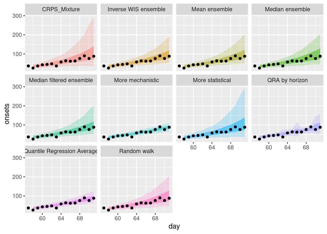

and on the log scale.

weighted_ensembles |>
  filter(origin_day == 57) |>
  plot_ensembles(onset_df |> filter(day >= 57, day <= 57 + 14)) +
  scale_y_log10()

Multiple forecasts

As before we can plot a range of forecasts from each model and ensemble.

plot_multiple_weighted_forecasts <- weighted_ensembles |>
  plot_ensembles(onset_df |> filter(day >= 21)) +
  lims(y = c(0, 400))
plot_multiple_weighted_forecasts

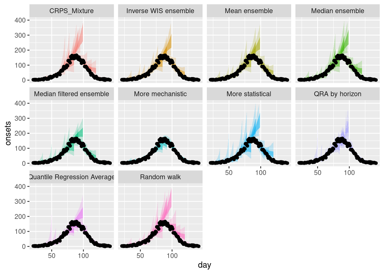
and on the log scale.

plot_multiple_weighted_forecasts +
  scale_y_log10()

Scale for y is already present.
Adding another scale for y, which will replace the existing scale.

Warning in scale_y_log10(): log-10 transformation introduced infinite values.
log-10 transformation introduced infinite values.
log-10 transformation introduced infinite values.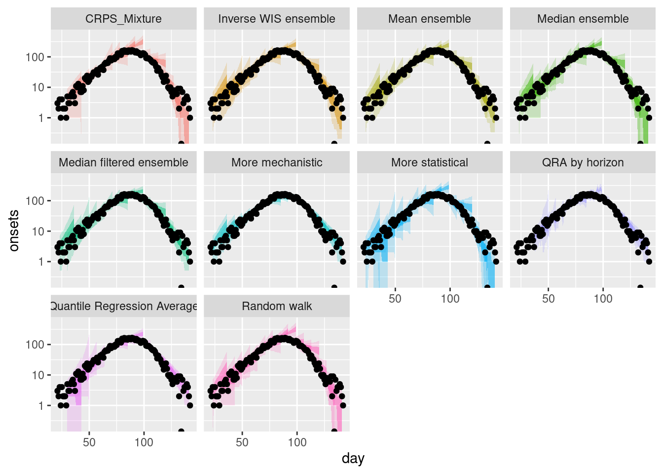

Take 2 minutes

How do the weighted ensembles compare to the simple ensembles? Which do you think is best? Are you surprised by the results? Can you think of any reasons that would explain them?

Solution

How do the weighted ensembles compare to the simple ensembles?

Model weights

We can also compare the weights that the different weighted ensembles we have created assign to each model.

weights <- rbind(
  weights_per_model |> mutate(method = "Inverse WIS"),
  qra_weights |> mutate(method = "QRA"),
  lop_weights |> mutate(method = "LOP")
)
weights |>
  ggplot(aes(x = origin_day, y = weight, fill = model)) +
  geom_col(position = "stack") +
  facet_grid(~ method) +
  theme(legend.position = "bottom")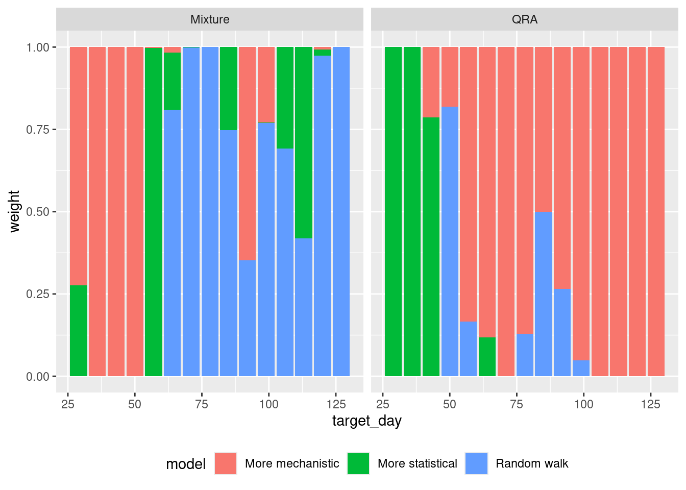

Take 2 minutes

Are the weights assigned to models different between the three methods? How do the weights change over time? Are you surprised by the results given what you know about the models performance?

Solution

Are the weights assigned to models different between the three methods?

• There are major differences especially early on, where the LOP ensemble prefers the random walk model and QRA the more statistical model.
• The inverse WIS model transitions from fairly even weights early on to giving most weights to the mechanistic model, however it does so in a more balanced manner than the optimised ensemble, giving substantial weight to all three models.

How do the weights change over time?

• Early on the more statistical models have higher weights in the respective ensemble methods.
• Gradually the mechanistic model gains weight in both models and by the end of the forecast horizon it represents the entire ensemble.

Are you surprised by the results given what you know about the models performance?

• As the random walk model is performing poorly, you would expect it to have low weights but actually it often doesn’t. This implies that its poor performance is restricted to certain parts of the outbreak.
• The mechanistic model performs really well overall and dominates the final optimised ensemble.

Evaluation

For a final evaluation we can look at the scores for each model and ensemble again. We remove the two weeks of forecasts as these do not have a quantile regression average forecasts as these require training data to estimate.

weighted_ensemble_scores <- weighted_ensembles |>
  filter(origin_day >= 29) |>
  as_forecast_quantile(forecast_unit = c("origin_day", "horizon", "model")) |>
  score()

Again we can get a high level overview of the scores by model.

weighted_ensemble_scores |>
  summarise_scores(by = c("model"))

                          model       wis overprediction underprediction
                         <char>     <num>          <num>           <num>
 1:        Inverse WIS ensemble  8.179605       3.739972       1.1895563
 2: Quantile Regression Average  7.438817       2.930858       2.1179392
 3:              QRA by horizon  8.006609       3.222753       2.2214614
 4:    Median filtered ensemble  7.255293       2.848571       1.5567143
 5:               Mean ensemble  8.709146       4.197524       1.1996825
 6:             Median ensemble 10.878952       5.954000       1.3623810
 7:                 Random walk 12.514186       7.376952       0.9014286
 8:            More statistical 11.595419       5.756476       1.8947619
 9:            More mechanistic  5.745548       1.568476       2.4212381
10:         Linear Opinion Pool  6.370671       1.275143       2.2822857
    dispersion        bias interval_coverage_50 interval_coverage_90 ae_median
         <num>       <num>                <num>                <num>     <num>
 1:   3.250076  0.18476190            0.5190476            0.8619048 12.544135
 2:   2.390020  0.07571429            0.4809524            0.7857143 11.436517
 3:   2.562395  0.12193878            0.4642857            0.7908163 12.215520
 4:   2.850007  0.09380952            0.5285714            0.8666667 11.121429
 5:   3.311940  0.14571429            0.5285714            0.8714286 13.284127
 6:   3.562571  0.10047619            0.5380952            0.8619048 16.600000
 7:   4.235805  0.16714286            0.5333333            0.8571429 19.085714
 8:   3.944181 -0.06809524            0.4952381            0.8428571 17.690476
 9:   1.755833  0.17571429            0.4809524            0.7714286  8.876190
10:   2.813243  0.03619048            0.5666667            0.8666667  9.390476

Remembering the session on forecast evaluation, we should also check performance on the log scale.

log_ensemble_scores <- weighted_ensembles |>
  filter(origin_day >= 29) |>
  as_forecast_quantile(forecast_unit = c("origin_day", "horizon", "model")) |>
    transform_forecasts(
    fun = log_shift,
    offset = 1,
    append = FALSE
  ) |>
  score()

log_ensemble_scores |>
  summarise_scores(by = c("model"))

                          model       wis overprediction underprediction
                         <char>     <num>          <num>           <num>
 1:        Inverse WIS ensemble 0.1660409     0.07773211      0.02514637
 2: Quantile Regression Average 0.1807427     0.08359583      0.03726745
 3:              QRA by horizon 0.1673600     0.08902760      0.02703905
 4:    Median filtered ensemble 0.1565710     0.06928781      0.02878697
 5:               Mean ensemble 0.1702717     0.07649681      0.02965817
 6:             Median ensemble 0.1930613     0.07919152      0.04153467
 7:                 Random walk 0.2059349     0.09204866      0.03774232
 8:            More statistical 0.2265978     0.06678145      0.07615982
 9:            More mechanistic 0.1612289     0.09838393      0.02188482
10:         Linear Opinion Pool 0.1627772     0.06745170      0.02915914
    dispersion        bias interval_coverage_50 interval_coverage_90 ae_median
         <num>       <num>                <num>                <num>     <num>
 1: 0.06316243  0.18476190            0.5190476            0.8619048 0.2535244
 2: 0.05987939  0.07809524            0.4809524            0.7857143 0.2719032
 3: 0.05129337  0.12448980            0.4744898            0.7908163 0.2469915
 4: 0.05849623  0.09380952            0.5285714            0.8666667 0.2397427
 5: 0.06411670  0.14571429            0.5285714            0.8714286 0.2602670
 6: 0.07233514  0.10047619            0.5380952            0.8619048 0.2978788
 7: 0.07614388  0.16714286            0.5333333            0.8571429 0.3172793
 8: 0.08365652 -0.06809524            0.4952381            0.8428571 0.3422939
 9: 0.04096012  0.17571429            0.4809524            0.7714286 0.2445859
10: 0.06616635  0.03619048            0.5666667            0.8666667 0.2415565

Take 2 minutes

How do the weighted ensembles compare to the simple ensembles on the natural and log scale?

Solution

The best ensembles slightly outperform some of the simple ensembles but there is no obvious benefit from using weighted ensembles. Why might this be the case?

Going further

Challenge

• Throughout the course we’ve been carefully building models from our understanding of the underlying data generating process. What might be the implications of combining models from different modellers, with different assumptions about this process? Think about the reliability and validity of the resulting ensemble forecast.
• Would it change how you approach communicating the forecast?

Methods in the real world

• Howerton et al. (2023) suggests that the choice of an ensemble method should be informed by an assumption about how to represent uncertainty between models: whether differences between component models is “noisy” variation around a single underlying distribution, or represents structural uncertainty about the system.
• Sherratt et al. (2023) investigates the performance of different ensembles in the European COVID-19 Forecast Hub.
• Amaral et al. (2025) discusses the challenges in improving on the predictive performance of simpler approaches using weighted ensembles.

Wrap up

• Review what you’ve learned in this session with the learning objectives
• Share your questions and thoughts

References

Amaral, André Victor Ribeiro, Daniel Wolffram, Paula Moraga, and Johannes Bracher. 2025. “Post-Processing and Weighted Combination of Infectious Disease Nowcasts.” PLoS Computational Biology 21 (3): e1012836. https://doi.org/10.1371/journal.pcbi.1012836.

Howerton, Emily, Michael C. Runge, Tiffany L. Bogich, Rebecca K. Borchering, Hidetoshi Inamine, Justin Lessler, Luke C. Mullany, et al. 2023. “Context-Dependent Representation of Within- and Between-Model Uncertainty: Aggregating Probabilistic Predictions in Infectious Disease Epidemiology.” Journal of The Royal Society Interface 20 (198): 20220659. https://doi.org/10.1098/rsif.2022.0659.

Sherratt, Katharine, Hugo Gruson, Rok Grah, Helen Johnson, Rene Niehus, Bastian Prasse, Frank Sandmann, et al. 2023. “Predictive Performance of Multi-Model Ensemble Forecasts of COVID-19 Across European Nations.” Edited by Amy Wesolowski, Neil M Ferguson, Jeffrey L Shaman, and Sen Pei. eLife 12 (April): e81916. https://doi.org/10.7554/eLife.81916.