Stan Reference

Quick reference for using Stan in this course

1. Why Stan in Epidemiology?

Uncertainty is an unavoidable part of real-world data
Need to estimate unobserved quantities (true cases, the effective reproduction number, future trends)
Bayesian approach naturally handles missing data and incorporates prior knowledge
Stan is a powerful tool for Bayesian inference

What is Stan?

Stan is a probabilistic programming language for Bayesian inference. It allows us to:

Write down models in a text file (ending .stan)
Generate samples from the posterior distribution using various methods (like Hamiltonian Monte Carlo)
Get proper uncertainty quantification for our estimates

We use Stan because: - We’ll need to estimate things (delays, reproduction numbers, case numbers now and in the future) - We’ll want to correctly specify uncertainty - We’ll want to incorporate our domain expertise - We’ll do this using Bayesian inference

2. Just Enough Probability

What is a Probability Distribution?

A probability distribution describes how likely different outcomes are for a random variable.

Discrete distributions (for countable outcomes): - Example: Number of horse kick deaths per year (0, 1, 2, 3, …) - Poisson distribution with \(\lambda\) = 0.61 kicks per year - Probability of exactly 2 deaths: dpois(2, lambda = 0.61) = 0.11

Continuous distributions (for measurable quantities): - Example: Temperature in Stockholm tomorrow - Normal distribution with mean 23°C, standard deviation 2°C - Probability density at 30°C: dnorm(30, mean = 23, sd = 2) = 0.0001

Two Key Operations

Calculate probability/density: Given parameters, what’s the probability of observing a value?
Generate samples: Given parameters, simulate random observations

Distributions You’ll See

Distribution	Used for	Parameters	Example
Log-normal	Delays (e.g., incubation period)	meanlog, sdlog	Symptom onset time
Gamma	Delays (alternative)	shape, rate	Hospital length of stay
Negative Binomial	Count data with overdispersion	mu, phi	Daily case counts
Normal	Continuous measurements	mean, sd	Log(Rt)
Beta	Proportions	alpha, beta	Reporting probability

Key Concept: Parameters vs Data

Data: What we observe (onset dates, test results)
Parameters: What we want to learn (mean delay, Rt)
Model: How parameters generate data

Bayesian Inference in a Nutshell

The generative model can produce output which looks like data given a set of parameters \(\theta\)

Idea of Bayesian inference: treat \(\theta\) as random variables (with a probability distribution) and condition on data: posterior probability p(\(\theta\) | data) as target of inference.

Using Bayes’ rule: \[p(\theta | \text{data}) = \frac{p(\text{data} | \theta) p(\theta)}{p(\text{data})}\]

p(data | θ) is the likelihood
p(θ) is the prior
p(data) is a normalisation constant

In words: (posterior) ∝ (normalised likelihood) × (prior)

MCMC: Getting Samples from the Posterior

Markov-chain Monte Carlo (MCMC) is a method to generate samples of \(\theta\) that come from the posterior distribution given data. This is our target of inference.

Many flavours of MCMC exist:

Metropolis-Hastings
Hamiltonian Monte Carlo (what Stan uses)
Gibbs sampling

Stan uses the No-U-TURN sampler a form of Hamiltonian Monte Carlo sampler to efficiently explore the posterior distribution and generate samples. This has been shown to be efficient across a wide range of models It’s main limitation is that it doesn’t support discrete latent parameters.

3. Stan Basics for This Course

Model Structure

Every Stan model has three essential blocks:

data {
  // What we observe
  int<lower=0> N;  // number of observations
  array[N] real y; // the observations
}

parameters {
  // What we want to estimate
  real<lower=0> mean_delay;
  real<lower=0> sd_delay;
}

model {
  // How parameters relate to data
  // Prior
  mean_delay ~ normal(5, 2);
  sd_delay ~ normal(2, 1);
  
  // Likelihood
  y ~ lognormal(log(mean_delay), sd_delay);
}

Running Stan from R

library(cmdstanr)
library(nfidd)

# Load a model
model <- nfidd_cmdstan_model("delays")

# Prepare data
stan_data <- list(
  N = length(observations),
  y = observations
)

# Fit model
fit <- nfidd_sample(model, data = stan_data)

# Extract results
summarise_draws(fit)

4. Debugging Tips

Check Your Priors

Do your priors make sense?
What range of predictions do they lead to?
Does this make sense for the data you’re modelling?

Before fitting your model, simulate from your priors to check they make sense:

# Example: checking delay priors
prior_mean_delay <- abs(rnorm(1000, mean = 1.5, sd = 0.5))
prior_sd_delay <- abs(rnorm(1000, mean = 0.5, sd = 0.1))

# Simulate delays from these priors
prior_delays <- rlnorm(
  1000, 
  meanlog = log(prior_mean_delay), 
  sdlog = prior_sd_delay
)

# Plot to check if reasonable
hist(prior_delays, breaks = 50)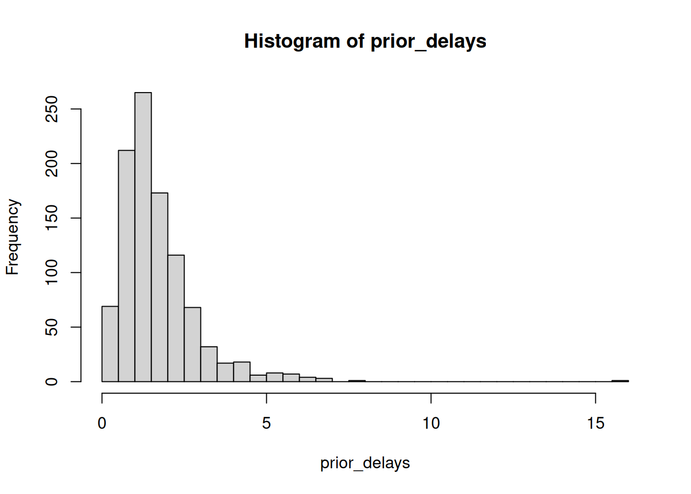

quantile(prior_delays, c(0.025, 0.5, 0.975))

     2.5%       50%     97.5% 
0.3449775 1.4106671 4.7809697

Check your model

Does your model make sense?
Does it have the parameters you expect?
Does it have the data you expect?

Check your data

Does your data make sense?
Does it have the variables you expect?
Does it have the right number of observations?

Check your results

Does your model fit the data?
Do the parameter estimates make sense?

Use posterior predictive checks to see if your model can reproduce data similar to what you observed: - Does it capture the central tendency of the data? - Does it get the right amount of variability? - Can it reproduce extreme values appropriately?

Compare your posterior predictions to the observed data using density overlays, empirical CDFs, and summary statistics.

Common Issues & Solutions

Issue	Symptom	What	Solution
Divergent transitions	Warning message	Sampler can’t explore posterior due to geometry of the posterior	Increase adapt_delta
Treedepth	Warning message	Sampler hit maximum tree depth before completing trajectory (complex posterior geometry requires longer integration paths)	Increase max_treedepth (e.g., to 12 or 15)
Low ESS	ESS < 400	Poor mixing between chains	Run more iterations
High Rhat	Rhat > 1.01	Chains sampling different distributions (not converged)	Check model specification or run more warmup iterations
Initialization failed	Error on startup	Numerical instability at start	Set init values

Understanding Divergences

Divergent transitions occur when the sampler encounters regions of the posterior that are difficult to explore. This often happens when:

The posterior has areas of high curvature
Parameters are on very different scales
There are strong correlations between parameters

Solutions:

# Increase adapt_delta (default is 0.8)
fit <- nfidd_sample(
  model, 
  data = stan_data,
  adapt_delta = 0.95  # or even 0.99 for difficult models
)